Interest Rate acquisition, and Forward Rate computation in R
In this post, we will use the R-package FRBData, (Takayanagi, 2011) to fetch interest rate data from the internet, plots its term structure, and compute the forward discount count.
Fetching the data
The FRBData package provides functions which can get financial and economical data from Federal Reserve Bank's website. For information regarding the day count convention and the compounding frequency of IR curves, read the footnote on the website.
For example, in order to get the SWAP curve, for a specific range of dates, we would type the following in the the R termial
library(FRBData)

ir_swp_rates <- GetInterestRates(id = "SWAPS",from = as.Date("2014/06/11"), to = as.Date("2014/06/30"))
For the rest of this post, we will use the Constant Maturity Rate
Constant Maturity Rate
CMT yields are read directly from the Treasury's daily yield curve and represent "bond equivalent yields" for securities that pay semiannual interest, which are expressed on a simple annualized basis. As such, these yields are not effective annualized yields or Annualized Percentage Yields (APY), which include the effect of compounding. To convert a CMT yield to an APY you need to apply the standard financial formula:
APY = (1 + CMT/2)^2 -1
Treasury does not publish the weekly, monthly or annual averages of these yields. However, the Board of Governors of the Federal Reserve System also publishes these rates on our behalf in their Statistical Release H.15. The web site for the H.15 includes links that have the weekly, monthly and annual averages for the CMT indexes
Similar to the SWAP rate example above, in order to get the CMT rates into R, we use the following command
# Constant maturity yield curve
ir_const_maturities <- GetInterestRates(id = "TCMNOM",lastObs = 11)
Note that in the above example, instead of specifying a date range, we are opting to fetch the last 11 observations.
Plotting a term structure for a specific day
The following code was inspirerd by the one provided by (Hanson, 2014). For the plot, we will use the R-package ggplot2 (Wickham, 2009)
library(ggplot2)
i <- 10
term_str <- t(ir_const_maturities[i, ])
ad <- index(ir_const_maturities)[i] # anchor date

# Plotting the term structure
df.tmp <- data.frame(term = 1:length(ir_const_maturities[i, ]), rates  = t(coredata(ir_const_maturities[i, ])))
gplot <- ggplot(data = df.tmp, aes(x = term, y = rates)) + geom_line() +geom_point()
gplot <- gplot + scale_x_discrete(breaks=df.tmp$term, labels=colnames(ir_const_maturities))
gplot <- gplot + ggtitle(paste("Market Zero Rates for:", ad)) + xlab("Term") + ylab("Rates (%)")
gplot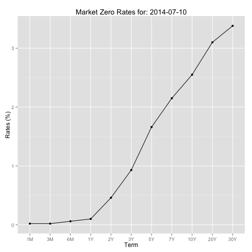
Yield Curve Construction
The first step is to construct the term-axis based on the columns names of the obtained data. To facilitate the construction of the various date, we will be using the lubridate package (Grolemund and Wickham, 2011)
library(lubridate)
term.str.dt <- c()
for (j in colnames(ir_const_maturities)) {
  term_num <- as.numeric(substring(j, 1, nchar(j) - 1))
  term <- switch(tolower(substring(j, nchar(j))),
                 "y" = years(term_num),
                 "m" = months(term_num),
                 "w" = weeks(term_num),
                 stop("Unit unrecognized in the term structure file"))
  term.str.dt <- cbind(term.str.dt, ad + term)
}
term.str.dt <- as.Date(term.str.dt, origin = "1970-01-01")
Next step is we construct the curve for the most recent date
require(xts)
ad <- index(last(ir_const_maturities))
rates <- t(coredata(last(ir_const_maturities))) * 0.01 # converting the decimal from percentage
# Make sure that the data is monotone - it's NOT always the case, since these data are weekly averages and not directly observed
if (any(rates != cummax(rates))) {
  # Checks if the data is montonoe, if not fix it
  for (t in 2:length(rates)) {
    if (rates[t] < rates[t-1]) rates[t] = rates[t-1]
  }
}
As mentioned in the above comments, we have to make sure that the IR data is monotonically increasing - otherwise we obtain a negative forward rate which will result in arbitrage opportunity. In order to do so, we cummax function as described in (Ali, 2012)
Next, we will use the xts package (Ryan and Ulrich, 2014) to construct and represent the zero curve
zcurve <- as.xts(x = rates, order.by = term.str.dt)

seq.date <- seq.Date(from = index(last(ir_const_maturities)), to = last(index(zcurve)), by = 1)
term.str.dt.daily <- xts(order.by= seq.date)

zcurve <- merge(zcurve, term.str.dt.daily)
Next we interpolate the data in between. In the following example we will use two interpolation methods: linear and cubic spline
zcurve_linear <- na.approx(zcurve) # Linear interpolation
zcurve_spline <- na.spline(zcurve, method = "hyman") # Spline interpolation which guarentees monotone output
colnames(zcurve_spline) <- NULL
zcurve_spline <- na.locf(zcurve_spline, na.rm = FALSE, fromLast = TRUE) # flat extrapolation to the left
Plotting the interpolated curve
library(scales) # needed for the date_format() function
df.tmp <- data.frame(term = index(zcurve_spline), rates = coredata(zcurve_spline))
gplot <- ggplot(data = df.tmp, aes(x = term, y = rates)) + geom_line()
gplot <- gplot + scale_x_date(labels = date_format())
gplot <- gplot + theme(axis.text.x = element_text(angle = 90, vjust = 0.5, hjust=1))
gplot <- gplot + ggtitle(paste("Market Zero Rates for:", ad)) + xlab("Term") + ylab("Rates (%)")
gplot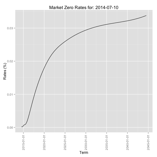
Note: In order to see the impact of using the default cubic spline method, instead of the using method = "hyman", the reader should refer to (Ali, 2012)
Construction of the forward curves and taking Day Count Convention into account
The code for the this section is borrowed from (Hanson, 2014)
First step is the construction of the function that computes the fraction of a year, based on the day count convention of the curve. We illustrate this by construction a code that uses ACT/365 days count convention
delta_t_Act365 <- function(from_date, to_date){
  if (from_date > to_date)
    stop("the 2nd parameters(to_date) has to be larger/more in the future than 1st paramters(from_date)")
  yearFraction <- as.numeric((to_date - from_date)/365)
  return(yearFraction)
}
Next we construct the forward discount factor based on the day count convention, and using the function we just defined
fwdDiscountFactor <- function(t0, from_date, to_date, zcurve.xts, dayCountFunction) {
  if (from_date > to_date)
    stop("the 2nd parameters(to_date) has to be larger/more in the future than 1st paramters(from_date)")
  rate1 <- as.numeric(zcurve.xts[from_date])      # R(0, T1)
  rate2 <- as.numeric(zcurve.xts[to_date])        # R(0, T2)
  # Computing discount factor
  discFactor1 <- exp(-rate1 * dayCountFunction(t0, from_date))
  discFactor2 <- exp(-rate1 * dayCountFunction(t0, to_date))

  fwdDF <- discFactor2/discFactor1
  return(fwdDF)
}
Finally we compute the forward zero curve, again using the day count convention function we have defined above
fwdInterestRate <- function(t0, from_date, to_date, zcurve.xts, dayCountFunction) {
  # we are passing the zero curve, because we will compute the discount factor inside this function
  if (from_date > to_date)
    stop("the 2nd parameters(to_date) has to be larger/more in the future than 1st paramters(from_date)")
  else if (from_date == to_date)
    return(0)
  else {
    fwdDF <- fwdDiscountFactor(t0, from_date, to_date, zcurve.xts, dayCountFunction)
    fwdRate <- -log(fwdDF)/dayCountFunction(from_date, to_date)
  }
  return(fwdRate)
}
Examples
Putting it all together, in order to use the above code to compute the forward discount factor/rate, observed at time t0, we would use the following code
t0 <- index(last(ir_const_maturities))

fwDisc <- fwdDiscountFactor(t0, from_date = t0 + years(5), to_date = t0 + years(10),
                            zcurve.xts = zcurve_spline, dayCountFunction = delta_t_Act365)

fwrate <- fwdInterestRate(t0, from_date = t0 + years(5), to_date = t0 + years(10),
                          zcurve.xts = zcurve_spline, dayCountFunction = delta_t_Act365)
Validation examples:
# Test 1: Trivial case
fwdDiscountFactor(t0, from_date = t0 + years(5), to_date = t0 + years(5),
                  zcurve.xts = zcurve_spline, dayCountFunction = delta_t_Act365)
## [1] 1fwdInterestRate(t0, from_date = t0 + years(5), to_date = t0 + years(5),
zcurve.xts = zcurve_spline, dayCountFunction = delta_t_Act365)## [1] 0# Test 2: Recovering the original interest rate
setting the start date to equal t0
tt1 <- fwdInterestRate(t0, from_date = t0, to_date = t0 + months(1),
                       zcurve.xts = zcurve_spline, dayCountFunction = delta_t_Act365)
tt2 <- coredata(last(ir_const_maturities))[,"1M"] * 0.01 # since the orginial was in decimal format
Checking that the two values are "equal"
all.equal(tt1, tt2, check.attributes = FALSE, tolerance = .Machine$double.eps)## [1] "Mean relative difference: 1.458e-12"This value is accurate enough and is smaller than the default threshold of all.equal function
References
Citations made with knitcitations (Boettiger, 2014).
[1] Ali. How to check if a sequence of numbers is monotonically increasing (or decreasing)?. 2012. URL: http://stackoverflow.com/questions/13093912/how-to-check-if-a-sequence-of-numbers-is-monotonically-increasing-or-decreasing.
[2] C. Boettiger. knitcitations: Citations for knitr markdown files. R package version 1.0-1. 2014. URL: https://github.com/cboettig/knitcitations.
[3] G. Grolemund and H. Wickham. "Dates and Times Made Easy with lubridate". In: Journal of Statistical Software 40.3 (2011), pp. 1-25. URL: http://www.jstatsoft.org/v40/i03/.
[4] D. Hanson. Quantitative Finance Applications in R - 6: Constructing a Term Structure of Interest Rates Using R (Part 1). 2014. URL: http://blog.revolutionanalytics.com/2014/06/quantitative-finance-applications-in-r-6-constructing-a-term-structure-of-interest-rates-using-r-par.html.
[5] D. Hanson. Quantitative Finance applications in R - 7: Constructing a Term Structure of Interest Rates Using R (part 2 of 2). 2014. URL: http://blog.revolutionanalytics.com/2014/07/quantitative-finance-applications-in-r-7-constructing-a-term-structure-of-interest-rates-using-r-par.html.
[6] J. A. Ryan and J. M. Ulrich. xts: eXtensible Time Series. R package version 0.9-7. 2014. URL: http://CRAN.R-project.org/package=xts.
[7] S. Takayanagi. FRBData: Download interest rate data from FRB's website. R package version 0.3. 2011. URL: http://CRAN.R-project.org/package=FRBData.
[8] H. Wickham. ggplot2: elegant graphics for data analysis. Springer New York, 2009. ISBN: 978-0-387-98140-6. URL: http://had.co.nz/ggplot2/book.
Reproducibility
sessionInfo()## R version 3.1.1 (2014-07-10)
## Platform: x86_64-apple-darwin10.8.0 (64-bit)
##
## locale:
## [1] en_CA.UTF-8/en_CA.UTF-8/en_CA.UTF-8/C/en_CA.UTF-8/en_CA.UTF-8
##
## attached base packages:
## [1] stats graphics grDevices utils datasets methods base
##
## other attached packages:
## [1] scales_0.2.4 lubridate_1.3.3 ggplot2_1.0.0
## [4] FRBData_0.3 xts_0.9-7 zoo_1.7-11
## [7] bibtex_0.3-6 knitr_1.6 RefManageR_0.8.2
## [10] knitcitations_1.0-1
##
## loaded via a namespace (and not attached):
## [1] codetools_0.2-8 colorspace_1.2-4 digest_0.6.4 evaluate_0.5.5
## [5] formatR_0.10 grid_3.1.1 gtable_0.1.2 httr_0.3
## [9] labeling_0.2 lattice_0.20-29 MASS_7.3-33 memoise_0.2.1
## [13] munsell_0.4.2 plyr_1.8.1 proto_0.3-10 Rcpp_0.11.2
## [17] RCurl_1.95-4.1 reshape2_1.4 RJSONIO_1.2-0.2 stringr_0.6.2
## [21] tools_3.1.1 XML_3.98-1.1