Who is Lalas? Lalas R Blog and Code
Linear State Space Linear Models, and Kalman Filters
Introduction
In this post, we will cover the topic of Linear State Space Models and the R-package, dlm(Petris, 2010). The example we cover are taken from the slides prepared by Eric Zivot and Guy Yollin; and the slides prepared by Giovanni Petris. The following are a list of topic covered:
- State Space Models
- Dynamics Linear Models
- Kalman Filters
- Numerical Examples
- Seemingly Unrelated Time Series Equations (SUTSE)
- Seemingly Unrelated Regression models
- Dynamic Common Factors Model
State Space Models
A State Space model, is composed of:
- Un-observable state: {\(x_0, x_1, x_2,..., x_t,...\)} which form a Markov Chain.
- Observable variable: {\(y_0, y_1, y_2,..., y_t,...\)} which are conditionally independent given the state.
It is specified by:
- \(p(x_o)\) which is initial distribution of states.
- \(p(x_t|x_{t-1})\) for \(t = 1, 2, 3 ...\) which is the transition probabilities of state from time \(t-1\) to \(t\)
- \(p(y_t|x_t)\) for \(t = 1, 2, 3 ...\) which is the conditional probability of the variable \(y\) at time \(t\); given that the state of the system, \(X\) at time \(t\).
Dynamics Linear Models
Dynamical Linear Models can be regarded as a special case of the state space model; where all the distributions are Gaussian. More specifically:
\[ \begin{align} x_0 \quad & \sim \quad N_p(m_0;C_0) \\ x_t|x_{t-1} \quad & \sim \quad N_p( G_t \, \cdot x_{t-1};W_t) \\ y_t|x_t \quad & \sim \quad N_m(F_t \cdot x_t;V_t) \\ \end{align} \]
where:
- \(F_t\) is a \(p \times m\) matrices
- \(G_t\) is a \(p \times p\) matrices
- \(V_t\) is a \(m \times m\) variance/co-variance matrix
- \(W_t\) is a \(p \times p\) variance/co variance matrix
Note that:
Often in the literature of State Space models, the symbol \(x_t\) and \(\theta_t\) are used interchangeably to refer to the state variable. For the rest of this tutorial, we will be using the symbol \(\theta\) unless otherwise specified.
Dynamics Linear Models in R
An equivalent formulation for a DLM is specified by the set of equations:
\[ \begin{align} y_t &= \, \, F_t \, \theta_t \, \, \, + \upsilon_t \qquad & \upsilon_t \sim N_m(0,V_t) \qquad & (1) \\ \theta_t &= \, G_t \, \theta_{t-1} + \omega_t\qquad & \omega_t \sim N_p(0,W_t) \qquad & (2) \\ \end{align} \]
for \(t = 1,...\) The specification of the model is completed by assigning a prior distribution for the initial (pre-sample) state \(\theta_0\).
\[ \begin{align} \theta_0 \quad \sim \quad N(m_0 ,C_0) \qquad \qquad \qquad \qquad \qquad \quad & (3) \end{align} \] That is a normal distribution with mean \(m_0\) and variance \(C_0\).
Note that:
- \(y_t\) and \(\theta_t\) are m and p dimensional random vectors, respectively
- \(F_t\), \(G_t\), \(V_t\) and \(W_t\) are real matrices of the appropriate dimensions.
- The sequences \(\upsilon_t\) and \(\omega_t\) are assumed to be independent, both within and between, and independent of \(\theta_0\).
- Equation (1) above, is called the measurement equation and it describes the vector of observations \(y_t\) through the signal \(\theta_t\) and a vector of disturbances \(\upsilon_t\)
- Equation (2) above, is called the transition equation and it describes the evolution of the state vector over time using a first order Markov structure.
In most applications, \(y_t\) is the value of an observable time series at time \(t\), while \(\theta_t\) is an unobservable state vector.
Time invariant models
In this model, the matrices \(F_t\), \(G_t\), \(V_t\), and \(W_t\) are constant and do NOT vary with time. Since they don't vary with time, we will drop the subscript \(t\).
Example 1: Random walk plus noise model (polynomial model of order one)
In this example the system of equations are \[ \begin{align} y_t &= \theta_t \quad + \upsilon_t \qquad & \upsilon_t \sim N(0,V) \\ \theta_t &= \theta_{ t-1 } \, + \omega_t \qquad & \omega_t \sim N(0,W) \\ \end{align} \]
Suppose one wants to define in R such a model, with \(V = 3.1\), \(W = 1.2\), \(m_0 = 0\), and \(C_0 = 100\). This can be done as follows:
library(dlm)
 myModel <- dlm(FF = 1, V = 3.1, GG = 1, W = 1.2, m0 = 0, C0 = 100)
where \(F_t\) (the FF parameters above), should be the identity matrix, but since \(p\) the number of dimension of \(\theta\) is equal to 1, \(F_t\) is reduced to 1. Similarly arguments goes for the \(G_t\) variable (the GG parameters above).
Time Varying DLM
A dlm object may contain, in addition to the components \(FF\), \(V\), \(GG\), \(W\), \(m0\), and \(C0\) described above, one or more of \(JFF\), \(JV\), \(JGG\), \(JW\), and \(X\). While \(X\) is a matrix used to store all the time-varying elements of the model, the components are indicator matrices whose entries signal whether an element of the corresponding model matrix is time-varying and, in case it is, where to retrieve its values in the matrix \(X\).
Example 2: Linear Regression (time varying parameters)
In the standard DLM representation of a simple linear regression models, the state vector is \(\theta_t = \left( \alpha_t\, ;\beta_t \right)^{\prime}\), the vector of regression coefficients, which may be constant or time-varying. In the case of time varying, the model is:
\[ \begin{align} y_t &= \alpha_t + \beta_t \, x_t + \epsilon_t \qquad & \epsilon_t \, \sim N(0,\sigma^2) \\ \alpha_t &= \quad \alpha_{t-1} \quad + \epsilon_t^{\alpha} \qquad & \epsilon_t^{\alpha} \sim N(0,\sigma_{\alpha}^2) \\ \beta_t &= \quad \beta_{t-1} \quad + \epsilon_t^{\beta} \qquad & \epsilon_t^{\beta} \sim N(0, \sigma_{\beta}^2) \\ \end{align} \] where
- \(\epsilon_t\), \(\epsilon_t^\alpha\) and \(\epsilon_t^\beta\) are iid
- The matrix \(F_t\) is [\(1 \, x_t\)] where \(x_t\) are value of the co-variate for observation \(y_t\)
- \(V\) is \(\sigma^{2}\)
More generally, a dynamic linear regression model is described by:
\[ \begin{align} y_t &= \mathbf{ x_t^\prime } \theta_t + v_t \qquad & \upsilon_t \sim N(0,V_t) \\ \theta_t &= \, G_t \, \theta_{t-1} + \omega_t \qquad & \omega_t \sim N(0,W_t) \\ \end{align} \]
where the coefficients:
- \(\mathbf{ x_t^{\prime} } := [x_{1t}, \dots , x_{pt}]\) are the p-explanatory variables at time \(t\). These are not assumed to be stochastic in this model, but rather fixed (i.e. this is a conditional model of \(y_t|x_t\)
- The system matrix \(G_t\) is the \(2×2\) identity matrix and
- the observation matrix is \(F_t\) = [\(1 \, x_t\)], where \(x_t\) is the value of the co-variate for observation \(y_t\).
A popular default choice for the state equation is to take the evolution matrix \(G_t\) as the identity matrix and \(W\) diagonal, which corresponds to modeling the regression coefficients as independent random walks
Assuming the variances \(V_t\) and \(W_t\) are constant, the only time-varying element of the model is the \((1, 2)^{th}\) entry of \(F_t\).
Accordingly, the component \(X\) in the dlm object will be a one-column matrix containing the values of the co-variate \(x_t\), while \(JFF\) will be the \(1 \times 2\) matrix [0 1], where the ‘0’ signals that the \((1, 1)^{th}\) component of \(F_t\) is constant, and the ‘1’ means that the \((1, 2)^{th}\) component is time-varying and its values at different times can be found in the first column of \(X\).
Example 3: Local Linear Trend
In example 1, we described the random walk plus noise model, also called polynomial model of order one. In this example, we examine the local linear trend model, also called polymonial model of order two, which is described by the following set of equations:
\[ \begin{align} y_t &= \qquad \quad \mu_t + \upsilon_t \quad &\upsilon_t \sim N(0,V) \\ \mu_t &= \mu_{t-1} + \delta_{t-1} + \omega_t^{\mu} \quad & \omega_t^{\mu} \sim N(0,W^{\mu}) \\ \delta_t &= \qquad \,\, \, \delta_{t-1} + \omega_t^{\delta} \quad & \omega_t^{\delta} \sim N(0,W^{\delta}) \\ \end{align} \]
This model is used to describes dynamic of “straight line” observed with noise. Hence
- levels \(\mu_t\) which are locally linear function of time
- straight line if \(W^\mu\) and \(W^\delta\) are equal to 0
- When \(W^\mu\) is 0; \(\mu\) follows an integrated random walk
Signal-to-Noise Ratio
In the case where \(m = p = 1\) where m and p are the dimension of the variance matrices, \(V\) and \(W\) respectively; we can define the signal-to-noise ratio as being \(W_t/V_t\) where \(W_t\) is the evolution variance of the state \(\theta\) from \(t\) to \(t+1\) and \(V_t\) is the variance of observation given the state.
Dynamic Linear Model package.
In this section we will examine some of the functions used in the DLM R package. Using this package, a user can define the Random Walk plus noise model using the dlmModPoly helper function as follows:
myModel <- dlmModPoly(order = 1, dV = 3.1, dW = 1.2, C0 = 100)Other helpers function exist for more complex models such as:
dlmModARMA: for an ARMA process, potentially multivariatedlmModPoly: for an \(n^{th}\) order polynomialdlmModReg: for Linear regressiondlmModSeas: for periodic – Seasonal factorsdlmModTrig: for periodic – Trigonometric form
sum of DLM
The previous helper function can be combined to create a more complex models. For example:
myModel <- dlmModPoly(2) + dlmModSeas(4)creates a Dynamical Linear Model representing a time series for quarterly data, in which one wants to include a local linear trend (polynomial model of order 2) and a seasonal component.
Outter sum of DLM
Also Two DLMs, modeling an m1- and an m2-variate time series respectively, can also be combined into a unique DLM for m1 + m2- variate observations. For example
bivarMod <- myModel %+% myModelcreates two univariate models for a local trend plus a quarterly seasonal component as the one described above can be combined as follows (here m1 = m2 = 1). In this case the user has to be careful to specify meaningful values for the variances of the resulting model after model combination.
Both sums and outer sums of DLMs can be iterated and they can be combined to allow the specification of more complex models for multivariate data from simple standard univariate models.
Setting and Getting component of models
- In order to fetch or set a component of a model defined, one can use the function \(FF\), \(V\), \(GG\), \(W\), \(m0\), and \(C0\).
- If the model have time varying parameters, these could accessed through the \(JFF\), \(JV\), \(JGG\), \(JW\), and \(X\).
For example:
V(myModel)
m0(myModel) <- rnorm()
Kalman Filters
Filtering:
Let \( y^t = (y_1, ..., y_t) \) be the vector of observation up to time \(t\). The filtering distributions, \(p(\theta_t|y^{t})\) can be computed recursively as follows:
Start with \( \theta_0 \sim N(m_0, C_0) \) at time 0
One step forecast for the state \[ \theta_t|y^{t-1} \sim N(a_t, R_t) \] where \(a_t = G_t \cdot m_{t-1} \), and \(R_t = G_t C_{t-1} G_t^\prime + W_t\)
One step forecast for the observation \[ y_t|y^{t-1} \sim N(f_t, Q_t) \] where \(f_t = F_t \cdot a_t\), and \(Q_t = F_t R_{t-1} F_t^\prime + V_t\)
Compute the posterior at time \(t\); \[ \theta_t|y^t \sim N(m_t, C_t) \] where \(m_t = a_t + R_t \, f_t^\prime Q_t^{-1} (y_t - f_t)\), and \(C_t = R_t - R_t F_t^\prime Q_t^{-1} F_t R_t\)
Filtering in the DLM package
The function dlmFilter returns:
- the series of filtering means \(m_t = E(\theta_t|y^{t})\) – includes \(t = 0\)
- the series of filtering variances \(C_t = Var(\theta_t|y^{t})\) – includes \(t = 0\)
- the series of one-step forecasts for the state \(a_t = E(\theta_t|y^{t−1})\)
- the series of one-step forecast variances for the state \(R_t = Var(\theta_t|y^{t−1})\)
- the series of one-step forecasts for the observation \(f_t = E(y_t|y^{t−1})\)
Smoothing:
Backward recursive algorithm can be used to obtain \( p(\theta_t|y^T) \) for a fixed \(T\) and for \(t =\) {\(0, 1, 2, ...T\)}.
- Starting from \(\theta_T|y_T \sim N(m_T, C_T\) at time \(t = T\)
- For \(t\) in \(\left \{ T - 1, T - 2, ..., 0 \right \}\) \[ \theta_t|y^{T} \sim N(s_t, S_t) \] where: \[ \begin{align} s_t &= m_t + C_t \, G_{t+1}^{\, \prime} R_{t+1}^{-1}(s_{t+1} - a_{t + 1}) \qquad \textrm{and} \\ S_t &= C_t - C_t \, G_{t+1}^{\, \prime} R_{t+1}^{-1}(R_{t+1} - S_{t + 1}) \, R_{t+1}^{-1} G_{t+1}^{\, \prime} C_t \\ \end{align} \]
Smoothing in the DLM package
The function dlmSmooth returns:
- the series of smoothing means \( s_t = E(\theta_t|y^{T})\) – includes \(t = 0\)
- the series of smoothing variances \(S_t = Var(\theta_t|y^{T})\) – includes \(t = 0\)
Note that:
- Updating in Filtering is sequential which allows for online processing; while in Smoothing it is not; so processing is offline_
- The formulas shown above are numerically unstable, but other more stable algorithms are available; such as square-root filters. Package
dlmimplements a filter algorithm based on the singular value decomposition (SVD) of all the variance-co-variance matrices.
Forcasting:
To calculate the forecast distributions, for \(k = 1, 2, ...\) etc, we proceed as follows:
- starting with a sample from \(\theta_T|y_T \sim N(m_T, C_T)\)
Forecast the state: \[ \theta_{T+k}|y^{T} \sim N(a_k^{T}, R_k^{T}) \] where: \(a_t^{k} = G_{T+k} \, a_{k-1}^{T} \) and \( R_k^{T} = G_{T+k} \, R_{k-1}^{T} G_{T+k}^{\, \prime} + W_{T+k}\)
Forecast the observation: \[ \theta_{T+k}|y^T \sim N(f_k^{T}, Q_k^{T}) \] where: \(f_k^{T} = F_{T+k} \, a_k^{T} \) and \(Q_k^{T} = F_{T+k} \, R_k^{T} F_{T+k}^{\, \prime} + V_{T+k}\)
Residual Analysis and model checking
One way of verifying model assumption is to look at the model residuals. The One-step forecast errors, or innovations can be defined by \(e_t = y_t − E(y_t|y_{t−1})\). The innovations are a sequence of independent Gaussian random variables. These innovations can be used to obtain a sequence of i.i.d standard normal random variables as follows:
\[ \tilde {e_t} = \frac{e_t }{\sqrt{ Q_t } }\] where \(F_t = E(y_t|y^{t-1})\) and \(Q_t = \textrm{Var}(y_t|y^{t-1})\) are both estimates obtained from the Kalman Filter.
Notes about MLE estimation
Since we are estimating the parameters using the MLE method, there is not guarantee that the answer we obtain is the "optimal" solution. The common causes for this may be:
- Multiple local maxima of the log-likelihood
- Fairly flat log-likelihood surface
In order to gain confidence in the values return by the dlmMLE function, it's usually recommended that
- Repeat the optimization process several times, with different initial parameter values.
- Make sure the Hessian of the negative log-likelihood at the maximum is positive definite.
- Compute standard errors of MLEs to get a feeling for the accuracy of the estimates
One way of computing the Hessian matrix in R is to use the function hessian part of the numDeriv package. We will see a demonstration of this in example 5 below
Numerical Examples
Example 4: Regression Model
The next example are taking from the slides prepared by Eric Zivot and Guy Yollin. See slides 12-13 for more information.
First we load the data as such:
library(PerformanceAnalytics, quietly = TRUE,  warn.conflicts = FALSE)
data(managers)
# extract HAM1 and SP500 excess returns
HAM1 = 100*(managers[,"HAM1", drop=FALSE] - managers[,"US 3m TR", drop=FALSE])
sp500 = 100*(managers[,"SP500 TR", drop=FALSE] - managers[,"US 3m TR",drop=FALSE])
colnames(sp500) = "SP500"
Then we can proceed by specifying a dynamical regression model and its parameters
# Specifying a set model parameters
s2_obs = 1      # Variance of observations
s2_alpha = 0.01 # Variance of the alpha regression parameter
s2_beta = 0.01  # Variance of the beta regression parameter
# Construct a regression model
tvp.dlm = dlmModReg(X=sp500, addInt=TRUE, dV=s2_obs, dW=c(s2_alpha, s2_beta))
Now that we have define a model, we can view its different component:
# looking at the various component
tvp.dlm[c("FF","V","GG","W","m0","C0")]
tvp.dlm[c("JFF","JV","JGG","JW")]
If we were to do a simple linear regression (Ordinary Least Square fit - constant equity beta), we would do something like
ols.fit = lm(HAM1 ~ sp500)
summary(ols.fit)
##
## Call:
## lm(formula = HAM1 ~ sp500)
##
## Residuals:
## Min 1Q Median 3Q Max
## -5.178 -1.387 -0.215 1.263 5.744
##
## Coefficients:
## Estimate Std. Error t value Pr(>|t|)
## (Intercept) 0.5775 0.1697 3.40 0.00089 ***
## sp500 0.3901 0.0391 9.98 < 2e-16 ***
## ---
## Signif. codes: 0 '***' 0.001 '**' 0.01 '*' 0.05 '.' 0.1 ' ' 1
##
## Residual standard error: 1.93 on 130 degrees of freedom
## Multiple R-squared: 0.434, Adjusted R-squared: 0.43
## F-statistic: 99.6 on 1 and 130 DF, p-value: <2e-16In order to define and estimate this regression using dynamical system model, we would use the Maximum Likelihood Estimation (MLE) method to estimates the 3 parameters: s2_obs, s2_alpa and s2_beta. We first start by defining initial values for the estimation methods
start.vals = c(0,0,0)
# Names ln variance of: observation y, alpha and beta (corresponding intercept and slope of y (HAM1) with respect to X (sp500))
names(start.vals) = c("lns2_obs", "lns2_alpha", "lns2_beta")

# function to build Time Varying Parameter state space model
buildTVP <- function(parm, x.mat){
    parm <- exp(parm)
  return( dlmModReg(X=x.mat, dV=parm[1], dW=c(parm[2], parm[3])) )
}

# Estimate the model
TVP.mle = dlmMLE(y=HAM1, parm=start.vals, x.mat=sp500, build=buildTVP, hessian=T)

# get sd estimates
se2 <- sqrt(exp(TVP.mle$par))
names(se2) = c("s_obs", "s_alpha", "s_beta")
sqrt(se2)
## s_obs s_alpha s_beta
## 1.32902 0.03094 0.23528Now that we have an estimates for the model, we can build the "optimal" model using the estimates we obtained in the previous step.
# Build fitted ss model, passing to it sp500 as the matrix X in the model
TVP.dlm <- buildTVP(TVP.mle$par, sp500)
Filtering and Smooting:
- Filtering Optimal estimates of \(\theta_t\) given information available at time \(t\), \(I_t=\left \{ y_1,...,y_t \right\}\)
- Smoothing Optimal estimates of \(\theta_t\) given information available at time \(T\), \(I_T =\left \{ y_,...,y_T \right\}\)
Now that we have obtained model estimates, and build the optimal model, we can filter the data through it, to obtain filtered values of the state vectors, together with their variance/co-variance matrices.
TVP.f <- dlmFilter(y = HAM1, mod = TVP.dlm)
class(TVP.f)
## [1] "dlmFiltered"names(TVP.f)## [1] "y" "mod" "m" "U.C" "D.C" "a" "U.R" "D.R" "f"Similarly, to obtained the smoothed values of the state vectors, together with their variance/co-variance matrices; using knowledge of the entire series
# Optimal estimates of θ_t given information available at time T.
TVP.s <- dlmSmooth(TVP.f)
class(TVP.s)
## [1] "list"names(TVP.s)## [1] "s" "U.S" "D.S"Plotting the results (smoothed values)
Now that we have obtained the smoothed values of the state vectors, we can draw them as:
# extract smoothed states - intercept and slope coefs
alpha.s = xts(TVP.s$s[-1,1,drop=FALSE], as.Date(rownames(TVP.s$s[-1,])))
beta.s  = xts(TVP.s$s[-1,2,drop=FALSE], as.Date(rownames(TVP.s$s[-1,])))
colnames(alpha.s) = "alpha"
colnames(beta.s)  = "beta"
Extracting the std errors and constructing the confidence band
# extract std errors - dlmSvd2var gives list of MSE matrices
mse.list = dlmSvd2var(TVP.s$U.S, TVP.s$D.S)
se.mat = t(sapply(mse.list, FUN=function(x) sqrt(diag(x))))
se.xts = xts(se.mat[-1, ], index(beta.s))
colnames(se.xts) = c("alpha", "beta")
a.u = alpha.s + 1.96*se.xts[, "alpha"]
a.l = alpha.s - 1.96*se.xts[, "alpha"]
b.u = beta.s  + 1.96*se.xts[, "beta"]
b.l = beta.s  - 1.96*se.xts[, "beta"]
And plotting the results with +/- 2 times the standard deviation
# plot smoothed estimates with +/- 2*SE bands
chart.TimeSeries(cbind(alpha.s, a.l, a.u), main="Smoothed estimates of alpha", ylim=c(0,1),
                 colorset=c(1,2,2), lty=c(1,2,2),ylab=expression(alpha),xlab="")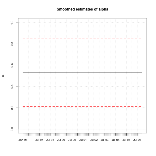
chart.TimeSeries(cbind(beta.s, b.l, b.u), main="Smoothed estimates of beta",
                 colorset=c(1,2,2), lty=c(1,2,2),ylab=expression(beta),xlab="")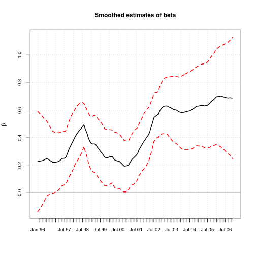
or using package ggplot2 (Saravia, 2012)
we would do
library(ggplot2, warn.conflicts = FALSE)
alpha.df <- data.frame(dateTime = index(se.xts), alpha = alpha.s, upr = a.u, lwr = a.l)
names(alpha.df) <- c("dateTime", "alpha", "upr", "lwr")
beta.df  <- data.frame(dateTime = index(se.xts), beta = beta.s, upr = b.u, lwr = b.l)
names(beta.df) <- c("dateTime", "beta", "upr", "lwr")
## Plotting alpha
ggplot(data = alpha.df, aes(dateTime, alpha) ) + geom_point () + geom_line() + geom_ribbon(data=alpha.df, aes(ymin=lwr,ymax=upr), alpha=0.3) + labs(x = "year", y = expression(alpha), title = expression(paste("State Space Values of ", alpha, " over Time")))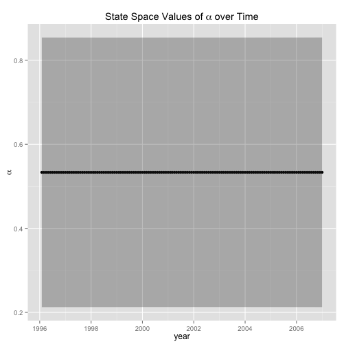
## Plotting beta
ggplot(data = beta.df, aes(dateTime, beta) ) + geom_point (data = beta.df, aes(dateTime, beta) ) + geom_line() + geom_ribbon(data=beta.df , aes(ymin=lwr,ymax=upr), alpha=0.3) + labs(x = "year", y = expression(beta), title = expression(paste("State Space Values of ", beta, " over Time")))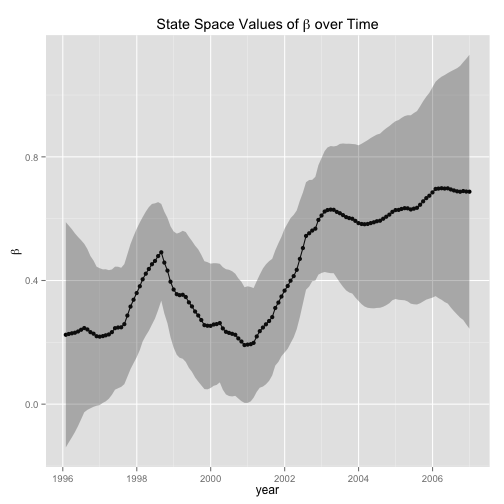
Forcasting using Kalman Filter
We will be doing a 10-steps ahead forecast using the calibrated model:
# Construct add 10 missing values to end of sample
new.xts = xts(rep(NA, 10), seq.Date(from=end(HAM1), by="months", length.out=11)[-1])
# Add this NA data to the original y (HAM1) series
HAM1.ext = merge(HAM1, new.xts)[,1]
# Filter extended y (HAM1) series
TVP.ext.f = dlmFilter(HAM1.ext, TVP.dlm)
# extract h-step ahead forecasts of state vector
TVP.ext.f$m[as.character(index(new.xts)),]
## [,1] [,2]
## 2007-01-31 0.5334 0.6873
## 2007-03-03 0.5334 0.6873
## 2007-03-31 0.5334 0.6873
## 2007-05-01 0.5334 0.6873
## 2007-05-31 0.5334 0.6873
## 2007-07-01 0.5334 0.6873
## 2007-07-31 0.5334 0.6873
## 2007-08-31 0.5334 0.6873
## 2007-10-01 0.5334 0.6873
## 2007-10-31 0.5334 0.6873We did not use the function dlmForecast part of the dlm package for future predictions, since that function works only with constant models!.
Residual Checkings
TVP.res <- residuals(TVP.f, sd = FALSE)
# Q-Q plot
qqnorm(TVP.res)
qqline(TVP.res)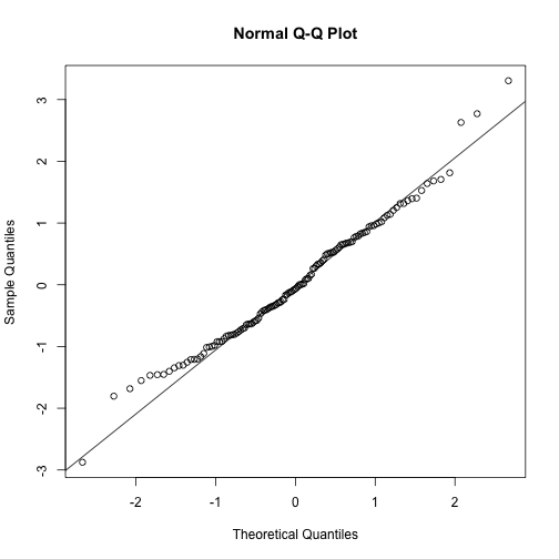
# Plotting Diagnostics for Time Series fits
tsdiag(TVP.f)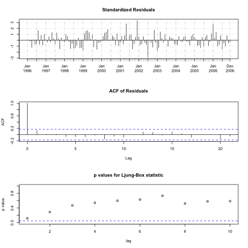
Example 5: Random Walk Plus noise - Nile River Data
We start this example by plotting the data set.
data(Nile)
Nile.df <- data.frame(year = index(Nile), y = as.numeric(Nile))
qplot(y = y, x = year, data = Nile.df, geom = 'line', ylab = 'Nile water level', xlab = 'Year',
                 main = "Measurements of the annual flow of \n the river Nile at Ashwan 1871-1970")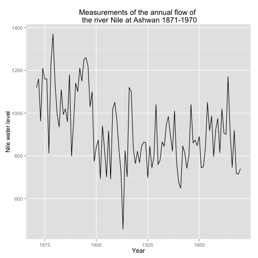
The previous graph illustrates the annual discharge of flow of water, (in unit of \(10^8\) \(m^3\), of the Nile at Aswan.
Next, we look at the effect of applying two different models with different Signal to Noise Ratio to the data, and see graphically, how well these two separate models fits the data (Pacomet, 2012).
# Creating models -- the variance V is the same in mod1 and mod2; but
# the signal variance is 10 time larger in mod2 than mod1
mod1 <- dlmModPoly(order = 1, dV = 15100, dW = 0.5 * 1468)
mod2 <- dlmModPoly(order = 1, dV = 15100, dW = 5 * 1468)
# Creating filter data
NileFilt_1 <- dlmFilter(Nile, mod1)
NileFilt_2 <- dlmFilter(Nile, mod2)
# Creating df to contain data to plot
Nile.df <- data.frame(year = index(Nile), Orig_data = as.numeric(Nile),
                      Filt_mod_1 = as.numeric(NileFilt_1$m[-1]), Filt_mod_2 = as.numeric(NileFilt_2$m[-1]))

# Plotting the results
library(wesanderson)
myColor <- wes.palette(3, "GrandBudapest")
p <- ggplot(data = Nile.df)
p <- p + geom_point(aes(x = year, y = Orig_data), size=3, colour= "black", shape = 21, fill = myColor[1])
p <- p + geom_line(aes(x = year, y = Orig_data,  colour = "Orig_data") , size = 1.0)
p <- p + geom_line(aes(x = year, y = Filt_mod_1, colour = "Filt_mod_1"), linetype="dotdash")
p <- p + geom_line(aes(x = year, y = Filt_mod_2, colour = "Filt_mod_2"), linetype="dotdash")
p <- p + labs(x = "year", y = "water Level", title = "Nile River water level for \n 2 different signal-to-noise ratios")
p <- p + scale_colour_manual("", breaks = c("Orig_data", "Filt_mod_1", "Filt_mod_2"),
                             labels= c("Org Data", "Filterd Data 1: SNR = x", "Filterd Data 2: SNR = 10x"),
                             values = myColor[c(2,3,1)])
p <- p + theme(legend.position="bottom")
print(p)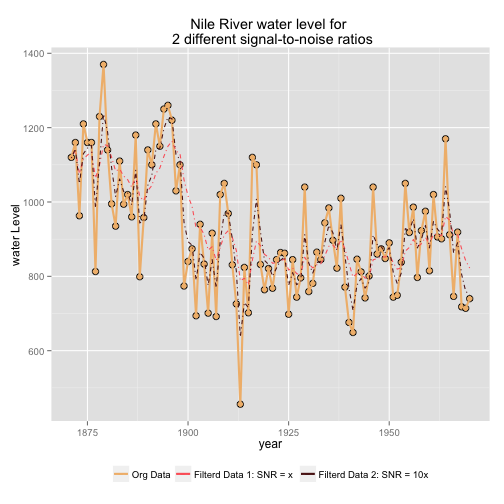
Next we fit a local level model, as described in example 1 above.
buildLocalLevel <- function(psi) dlmModPoly(order = 1, dV = psi[1], dW = psi[2])
mleOut <- dlmMLE(Nile, parm = c(0.2, 120), build = buildLocalLevel, lower = c(1e-7, 0))
# Checking that the MLE estimates has converged
mleOut$convergence
## [1] 0# Constructing the fitted model
LocalLevelmod <- buildLocalLevel(psi = mleOut$par)
# observation variance
drop(V(LocalLevelmod))## [1] 15100# system variance
drop(W(LocalLevelmod))## [1] 1468Note: The lower bound \(10^{-7}\) for \(V\) reflects the fact that the functions in dlm require the matrix \(V\) to be non-singular. On the scale of the data, however, \(10^{-7}\) can be considered zero for all practical purposes.
Looking at the plot of the original data, we notice a negative spike around the year 1900. This coincided with construction of the Aswan Low Dam, by the British during the years of 1898 to 1902. Recall that the model we just fit the data to (local level plus noise) assumes that the variance matrices \(W_t\) and \(V_T\) are constants over time. Therefore, one way to improve the accuracy of this model and take the jump in water level (around 1899) into account, is to assume that the variance did change on this year. The new model becomes: \[ \begin{align} y_t &= \theta_t + \upsilon_t \qquad & \upsilon_t \sim N(0,V)\\ \theta_t &= \, \theta_{ t-1 } + \omega_t \qquad & \omega_t \sim N(0,W_t)\\ \end{align} \]
where \[ W_t = \begin{cases} W \quad \,\,\, \textrm{if}\quad t \neq 1899 \\ W^*\quad \textrm{if}\quad t = 1899 \\ \end{cases} \]
We construct and estimate this model in R as follows:
# Model Construction
buildDamEffect <- function(psi) {
   mod <- dlmModPoly(1, dV = psi[1], C0 = 1e8)
   # Creating the X matrix for the model -- For more info see Time Varying DLM section above
   X(mod) <- matrix(psi[2], nr = length(Nile))
   X(mod)[time(Nile) == 1899] <- psi[3]
   # Tell R that the values of W_t at any time are to be found in the first column of the matrix X
   JW(mod) <- 1
   return(mod)
 }
# Model estimation through MLE
mleDamEffect <- dlmMLE(Nile, parm = c(0.2, 120, 20), build = buildDamEffect, lower = c(1e-7, 0, 0))
# Verify convergence
mleDamEffect$conv
## [1] 0# Construct the final model
damEffect <- buildDamEffect(psi = mleDamEffect$par)Finally, for the purpose of comparison, we build a Linear Trend model for the Nile data set
# Model Construction
buildLinearTrend <- function(psi) dlmModPoly(2, dV = psi[1], dW = psi[2:3], C0 = diag(1e8, 2))
# Model Estimation
mleLinearTrend <- dlmMLE(Nile, parm = c(0.2, 120, 20),build = buildLinearTrend, lower = c(1e-7, 0, 0))
# Checking convergence
mleLinearTrend$conv
## [1] 0# Construct Final Model
linearTrend <- buildLinearTrend(psi = mleLinearTrend$par)MLE results checking
We validate the results returned by the MLE method and gain confidence in the results by examining:
library(numDeriv)
# Local Level model
hs_localLevel <- hessian(function(x) dlmLL(Nile, buildLocalLevel(x)), mleOut$par)
all(eigen(hs_localLevel, only.values = TRUE)$values > 0) # positive definite?
## [1] TRUE# Damn Effect model
hs_damnEffect <- hessian(function(x) dlmLL(Nile, buildDamEffect(x)), mleDamEffect$par)
all(eigen(hs_damnEffect, only.values = TRUE)$values > 0) # positive definite?## [1] TRUE# Linear Trend model
hs_linearTrend <- hessian(function(x) dlmLL(Nile, buildLinearTrend(x)), mleLinearTrend$par)
all(eigen(hs_linearTrend, only.values = TRUE)$values > 0) # positive definite?## [1] TRUEModels Comparaison
Model selection for DLMs is usually based on either of the following criteria:
- Forecasting accuracy – such as Mean square error (MSE), Mean absolute deviation (MAD), Mean absolute percentage error (MAPE).
- Information criteria – such as AIC, BIC
- Bayes factors and posterior model probabilities (in a Bayesian setting)
If simulation is used, as it is the case in a Bayesian setting, then averages are calculated after discarding the burn-in samples (Petris, 2011).
In this next piece of code, we compute these various statistics
# Creating variable to hold the results
MSE <- MAD <- MAPE <- U <- logLik <- N <- AIC <- c()
# Calculating the filtered series for each model
LocalLevelmod_filtered <- dlmFilter(Nile, LocalLevelmod)
damEffect_filtered     <- dlmFilter(Nile, damEffect)
linearTrend_filtered   <- dlmFilter(Nile, linearTrend)
# Calculating the residuals
LocalLevel_resid  <- residuals(LocalLevelmod_filtered, type = "raw", sd = FALSE)
damEffect_resid   <- residuals(damEffect_filtered, type = "raw", sd = FALSE)
linearTrend_resid <- residuals(linearTrend_filtered , type = "raw", sd = FALSE)
# If sampling was obtained through simulation then we would remove the burn-in samples as in the next line
# linearTrend_resid <- tail(linearTrend_resid, -burn_in)
#
# Calculating statistics for different models:
# 1 LocalLevelmod
MSE["Local Level"] <- mean(LocalLevel_resid ^2)
MAD["Local Level"] <- mean(abs(LocalLevel_resid ))
MAPE["Local Level"] <- mean(abs(LocalLevel_resid) / as.numeric(Nile))
logLik["Local Level"] <- -mleOut$value
N["Local Level"] <- length(mleOut$par)
# 2 Dam Effect
MSE["Damn Effect"] <- mean(damEffect_resid^2)
MAD["Damn Effect"] <- mean(abs(damEffect_resid))
MAPE["Damn Effect"] <- mean(abs(damEffect_resid) / as.numeric(Nile))
logLik["Damn Effect"] <- -mleDamEffect$value
N["Damn Effect"] <- length(mleDamEffect$par)
# 3 linear trend
MSE["linear trend"] <- mean(linearTrend_resid^2)
MAD["linear trend"] <- mean(abs(linearTrend_resid))
MAPE["linear trend"] <- mean(abs(linearTrend_resid) / as.numeric(Nile))
logLik["linear trend"] <- -mleLinearTrend$value
N["linear trend"] <- length(mleLinearTrend$par)
# Calculating AIC and BIC- vectorized, for all models at once
AIC <- -2 * (logLik - N)
BIC <- -2 * logLik + N * log(length(Nile))
# Building a dataframe to store the results
results <- data.frame(MSE = MSE, MAD = MAD, MAPE = MAPE, logLik = logLik, AIC = AIC, BIC = BIC, NumParameter = N)
The following table summarize the results of the different model applied to the Nile data set.
# Producing a table
kable(results, digits=2, align = 'c')
##
##
## | | MSE | MAD | MAPE | logLik | AIC | BIC | NumParameter |
## |:------------|:-----:|:-----:|:----:|:------:|:----:|:----:|:------------:|
## |Local Level | 33026 | 123.7 | 0.14 | -549.7 | 1103 | 1109 | 2 |
## |Damn Effect | 30677 | 115.6 | 0.13 | -543.3 | 1093 | 1100 | 3 |
## |linear trend | 37927 | 133.6 | 0.15 | -558.2 | 1122 | 1130 | 3 |As we can the Damn Effect model is the best model out of the 3 models considered.
Seemingly Unrelated Time Series Equations (SUTSE)
SUTSE is a multivariate model used to describe univariate series that can be marginally modeled by the “same” DLM – same observation matrix \(F_0\) and system matrix \(G_0\), p-dimensional state vectors have the same interpretation.
For example, suppose there are \(k\) observed time series, each one might be modeled using a linear growth model, so that for each of them the state vector has a level and a slope component. Although not strictly required, it is commonly assumed for simplicity that the variance matrix of the system errors, \(W\) is diagonal. The system error of the dynamics of this common state vector will then be characterized by a block-diagonal variance matrix having a first \(k \times k\) block accounting for the correlation among levels and a second \(k \times k\) block accounting for the correlation among slopes. In order to introduce a further correlation between the \(k\) series, the observation error variance \(V\) can be taken non-diagonal.
Example
GDPs of different countries can all be described by a local linear trend – but obviously they are not independent For \(k\) such series, define the observation and system matrices of the joint model as:
\[ \begin{align} F &= F_0 \, \otimes \,I_k \\ G &= G_0 \, \otimes \,I_k \\ \end{align} \]
where \(I_k\) is the \(k \times k\) Identity matrix, and \(\otimes\) is the Kronecker product. The \(pk \times pk\) system variance \(W\) is typically given a block-diagonal form, with p \(k \times k\) blocks, implying a correlated evolution of the \(j^{th}\) components of the state vector of each series. The \(k \times k\) observation variance \(V\) may be non-diagonal to account for additional correlation among the different series.
Note: Given two matrices \(A\) and \(B\), of dimensions \(m \times n\) and \(p \times q\) respectively, the Kronecker product \(A \otimes B\) is the \(mp × nq\) matrix defined as:
\[ \begin{bmatrix} a_{11} \mathbf{B} & \cdots & a_{1n}\mathbf{B} \\ \vdots & \ddots & \vdots \\ a_{m1} \mathbf{B} & \cdots & a_{mn} \mathbf{B} \\ \end{bmatrix} \]
Example 6: GDP data
Consider GDP of Germany, UK, and USA. The series are obviously correlated and, for each of them – possibly on a log scale – a local linear trend model or possibly a more parsimonious integrated random walk plus noise seems a reasonable choice.
# We are unloading the namespace "ggplot2" since it mask the function %+% (outer sum) from the dlm package.
# http://stackoverflow.com/questions/3241539/how-to-unmask-a-function-in-r
unloadNamespace("ggplot2")
#
# Reading in the data
gdp0 <- read.table("http://definetti.uark.edu/~gpetris/UseR-2011/gdp.txt", skip = 3, header = TRUE)
# Transforming the data to the log-scale
gdp <- ts(10 * log(gdp0[, c("GERMANY", "UK", "USA")]), start = 1950)
# the ’base’ univariate model.
uni <- dlmModPoly() # Default paramters --> order = 2 --> stochastic linear trend.
# Creating an outter sum of models to  get the matrices of the correct dimension.
gdpSUTSE <- uni %+% uni %+% uni
# ## now redefine matrices to keep levels together and slopes together.
FF(gdpSUTSE) <- FF(uni) %x% diag(3)
GG(gdpSUTSE) <- GG(uni) %x% diag(3)
# ’CLEAN’ the system variance
W(gdpSUTSE)[] <- 0
#
# Define a “build” function to be given to MLE routine
buildSUTSE <- function(psi) {
 # Note log-Cholesky parametrization of the covariance matrix W
 U <- matrix(0, nrow = 3, ncol = 3)
 # putting random element in the upper triangle
 U[upper.tri(U)] <- psi[1 : 3]
 # making sure that the diagonal element of U are positive
 diag(U) <- exp(0.5 * psi[4 : 6])
 # Constructing the matrix W as the cross product of the U - equivalent to t(U) %*% U
 W(gdpSUTSE)[4 : 6, 4 : 6] <- crossprod(U)
 # parametrization of the covariance matrix V
 diag(V(gdpSUTSE)) <- exp(0.5 * psi[7 : 9])
 return(gdpSUTSE)
 }
#
# MLE estimate
gdpMLE <- dlmMLE(gdp, rep(-2, 9), buildSUTSE, control = list(maxit = 1000))
# Checking convergence
gdpMLE$conv
## [1] 0# Building the optimal model
gdpSUTSE <- buildSUTSE(gdpMLE$par)Note the log-Cholesky parametrization of the covariance matrix \(W\) (Pinheiro, 1994), in the buildSUTSE function. Looking at the estimated variance/covariance matrices:
W(gdpSUTSE)[4 : 6, 4 : 6]## [,1] [,2] [,3]
## [1,] 0.06080 0.02975 0.03246
## [2,] 0.02975 0.01756 0.02609
## [3,] 0.03246 0.02609 0.05200# correlations (slopes)
cov2cor(W(gdpSUTSE)[4 : 6, 4 : 6])## [,1] [,2] [,3]
## [1,] 1.0000 0.9104 0.5773
## [2,] 0.9104 1.0000 0.8634
## [3,] 0.5773 0.8634 1.0000# observation standard deviations
sqrt(diag(V(gdpSUTSE)))## [1] 0.04836 0.14746 0.12240#
# Looking at the smoothed series
gdpSmooth <- dlmSmooth(gdp, gdpSUTSE)The first three columns of gdpSmooth$s contain the time series of smoothed GDP level, the last three the smoothed slopes
Plotting the results
library(ggplot2)
library(reshape2)
# Preparing the data
# 1. Remove the first obs from the smoothed gdp,
#    since the time series, s, starts one time unit before the first observation.
level.df <- data.frame(year = index(gdp), gdpSmooth$s[-1,1:3])
# 2. naming the variable before melting the data
names(level.df)[2:4] <- colnames(gdp)
# 3. Melting the dataframe
level.df.melt = reshape2::melt(level.df, id=c("year"))
# Plotting the level
p <- ggplot(level.df.melt) + facet_grid(facets = variable ~ ., scales = "free_y")
p <- p + geom_line(aes(x=year, y=value, colour=variable)) + scale_colour_manual(values=myColor)
p <- p + labs(x = "year", y = expression(mu[t]), title = "The 'Smoothed' value of level of the state variable \n for log of the GDP per Capita")
p <- p + theme(legend.position="none")
print(p)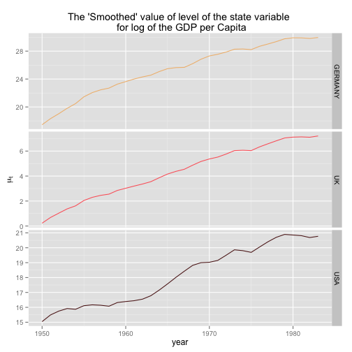
# Plotting the rate of change of the smoothed GDP per capita
slope.df <- data.frame(year = index(gdp), gdpSmooth$s[-1,4:6])
names(slope.df)[2:4] <- colnames(gdp)
slope.df.melt = reshape2::melt(slope.df, id=c("year"))
p <- ggplot(slope.df.melt) + facet_grid(facets = variable ~ ., scales = "free_y")
p <- p + geom_line(aes(x=year, y=value, colour=variable)) + scale_colour_manual(values=myColor)
p <- p + labs(x = "year", y = expression(delta[t]), title = "The 'Smoothed' value of Rate of Change of state variable \n for the log of the GDP per Capita")
p <- p + theme(legend.position="none")
print(p)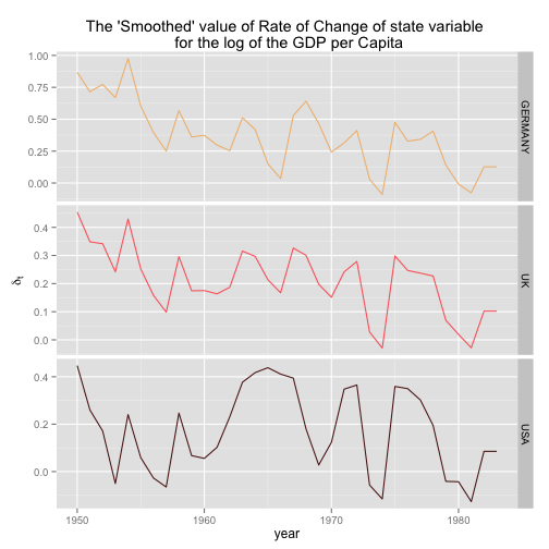
Seemingly Unrelated Regression models
Building on top of SUTSE, the next example we will consider is the multivariate version of the dynamic Capital Asset Pricing Model (CAPM) for \(m\) assets.
Let \({r_t}^{\,j} ,{r_t}^{\, M}\) and \({r_t}^{\, f}\) be the returns at time \(t\) of asset, \(j\), under study, of the market, \(M\), and of a risk-free asset, \(f\), respectively. Define the excess returns of the asset, \(j\) as \( y_{j,t} = r_{j,t} − r_t^{\, f}\) and the market’s excess returns as \(x_t = r_t^{\,M} − r_t^{\,f}\); where \(j = 1, \dots , m\). Then:
\[ \begin{align} y_{j,t} &= \alpha_{j,t} + \beta_{j,t} \, x_t + \upsilon_{j,t} \\ \alpha_{j,t} &= \alpha_{j,t-1} \qquad + \omega_{j,t}^\alpha \\ \beta_{j,t} &= \beta_{j,t-1} \qquad + \omega_{j,t}^\beta \\ \end{align} \]
where it is sensible to assume that the intercepts and the slopes are correlated across the $m$ stocks. The above model can be rewritten in a more general form such as
\[ \begin{align} \mathbf{y_t} &= (F_t \otimes I_m) \, \theta + \mathbf{\upsilon_t} \quad &\mathbf{\upsilon_t} \sim N(0,V)\\ \theta_t &= (G \otimes I_m) \, \theta_{t-1} + \mathbf{\omega_t} \quad &\mathbf{\omega_t} \sim N(0,W)\\ \end{align} \]
where
- \(\mathbf{y_t} = [y_{1t}, \dots , y_{mt}] \) are the values of the m different \(y\) series
- \(\theta_t = [\alpha_{1t}, \dots, \alpha_{mt}, \beta_{1p}, \dots, \beta_{mt}]\)
- \(\mathbf{\upsilon_t} = [\upsilon_{1t}, \dots, \upsilon_{mt}]\) and \(\mathbf{\omega_t} = [\omega_{1t}, \dots, \omega_{mt}]\) are iid
- \(W = \textrm{blockdiag}(W_{\alpha}; W_{\beta)}\)
- \(F_t = [1 \, x_t]\); and \(G = \textrm{I}_2\)
Example 7: CAPM regression model
We assume for simplicity that the \(\alpha_{j,t}\) are time-invariant, which amounts to assuming that \(W_{\alpha} = 0\).
data <- ts(read.table("http://shazam.econ.ubc.ca/intro/P.txt", header = TRUE),
           start = c(1978, 1), frequency = 12)
data <- data * 100
y <- data[, 1 : 4] - data[, "RKFREE"]
colnames(y) <- colnames(data)[1 : 4]
market <- data[, "MARKET"] - data[, "RKFREE"]
m <- NCOL(y)

# Define a “build” function to be given to MLE routine
buildSUR <- function(psi) {
  ### Set up the model
  CAPM <- dlmModReg(market, addInt = TRUE)
  CAPM$FF <- CAPM$FF %x% diag(m)
  CAPM$GG <- CAPM$GG %x% diag(m)
  CAPM$JFF <- CAPM$JFF %x% diag(m)
  # specifying the mean of the distribution of the initial state of theta (alpha; beta)
  CAPM$m0 <- c(rep(0,2*m))
  # Specifying the variance of the distribution of the initial state of theta (alpha; beta)
  CAPM$C0 <- CAPM$C0 %x% diag(m)
  # ’CLEAN’ the system and observation variance-covariance matrices
  CAPM$V <- CAPM$V %x% matrix(0, m, m)
  CAPM$W <- CAPM$W %x% matrix(0, m, m)
  #
  # parametrization of the covariance matrix W
  U <- matrix(0, nrow = m, ncol = m)
  # putting random element in the upper triangle
  U[upper.tri(U)] <- psi[1 : 6]
  # making sure that the diagonal element of U are positive
  diag(U) <- exp(0.5 * psi[7 : 10])
  # Constructing the matrix W_beta as the cross product of the U - equivalent to t(U) %*% U
  # Assuming W_alpha is zero
  W(CAPM)[5 : 8, 5 : 8] <- crossprod(U)
  # parametrization of the covariance matrix V
  U2 <- matrix(0, nrow = m, ncol = m)
  # putting random element in the upper triangle
  U2[upper.tri(U2)] <- psi[11 : 16]
  # making the diagonal element positive
  diag(U2) <- exp(0.5 * psi[17 : 20])
  V(CAPM) <- crossprod(U2)
  return(CAPM)
}

# MLE estimate
CAPM_MLE <- dlmMLE(y, rep(1, 20), buildSUR, control = list(maxit = 500))
# Checking convergence
CAPM_MLE$conv
## [1] 0# Build the model
CAPM_SUR <- buildSUR(CAPM_MLE$par)
# Looking at the estimated var-covariance of betas
W(CAPM_SUR)[5 : 8, 5 : 8]## [,1] [,2] [,3] [,4]
## [1,] 7.243e-06 9.768e-05 0.0001299 0.0002026
## [2,] 9.768e-05 1.326e-03 0.0017641 0.0027510
## [3,] 1.299e-04 1.764e-03 0.0023573 0.0036668
## [4,] 2.026e-04 2.751e-03 0.0036668 0.0057297# Viewing corr
cov2cor(W(CAPM_SUR)[5 : 8, 5 : 8])## [,1] [,2] [,3] [,4]
## [1,] 1.0000 0.9966 0.9943 0.9944
## [2,] 0.9966 1.0000 0.9976 0.9979
## [3,] 0.9943 0.9976 1.0000 0.9977
## [4,] 0.9944 0.9979 0.9977 1.0000# observation Variance Covariance
V(CAPM_SUR)## [,1] [,2] [,3] [,4]
## [1,] 41.03769 -0.01104 -0.9997 -2.389
## [2,] -0.01104 24.23393 5.7894 3.411
## [3,] -0.99971 5.78936 39.2327 8.161
## [4,] -2.38871 3.41080 8.1609 39.347# observation correlation
cov2cor(V(CAPM_SUR))## [,1] [,2] [,3] [,4]
## [1,] 1.0000000 -0.0003502 -0.02491 -0.05945
## [2,] -0.0003502 1.0000000 0.18776 0.11046
## [3,] -0.0249149 0.1877564 1.00000 0.20771
## [4,] -0.0594452 0.1104562 0.20771 1.00000# observation standard deviations
sqrt(diag(V(CAPM_SUR)))## [1] 6.406 4.923 6.264 6.273#
# Looking at the smoothed series
CAPM_Smooth <- dlmSmooth(y, CAPM_SUR)
#
# Plotting the result
myColor <- wes.palette(4, "GrandBudapest")
yr_seq <- seq(from = as.Date("1978-01-01"),to = as.Date("1987-12-01"), by = "months")
beta.df <- data.frame(year = yr_seq, CAPM_Smooth$s[-1, m + (1 : m)])
names(beta.df)[2:5] <- colnames(y)
beta.df.melt = reshape2::melt(beta.df, id=c("year"))
p <- ggplot(beta.df.melt) # + facet_grid(facets = variable ~ ., scales = "free_y")
p <- p + geom_line(aes(x=year, y=value, colour=variable)) + scale_colour_manual(values=myColor, name = "Stocks:")
p <- p + labs(x = "year", y = expression(beta[t]), title = expression(paste("The 'Smoothed' value of the ", beta, " in the CAPM model")))
p <- p + theme(legend.position="bottom" , axis.title.y = element_text(size=14))
print(p)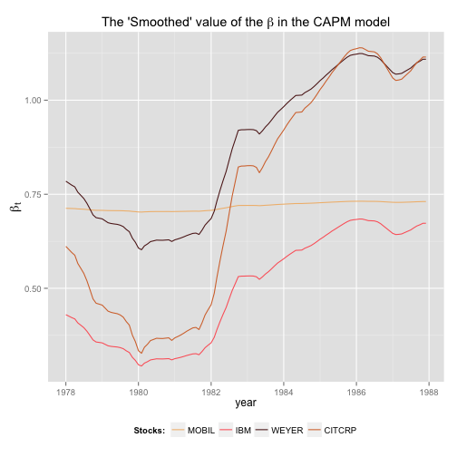
Dynamic Common Factors Model
Note: In this section we will use the parameter \(x\) instead of \(\theta\) to indicate the state since it's more common to use \(x\) as a variable in this kind of analysis.
Let \(y_t\) be an m-dimensional observation that can be modeled, at any time \(t\), as a linear combination of the factor components, \(z\), subject to additive observation noise. So: \[ y_t = A \, z_t + \upsilon_t \qquad \upsilon_t \sim N_m(0,V) \]
Let \(z_t\) be a q-dimensional vector of factors that evolves according to a DLM: \[ \begin{align} z_t &= F_0 \, x_t + \varepsilon_t \qquad & \varepsilon_t \sim N_q(0,\Sigma) \\ x_t &= G \, x_{t-1} + \omega_t \qquad & \omega_t \sim N_p(0,W) \\ \end{align} \]
Setting \(\Sigma = 0\) implies that \(\varepsilon_t = 0\) for every \(t\) and then we have
\[ \begin{align} y_t &= A \, F_0 \, x_t + \upsilon_t \qquad &\upsilon_t \sim N_m(0,V) \\ x_t &= \, \, G \, x_{t-1} + \omega_t \qquad & \omega_t\sim N_p(0,W) \\ \end{align} \]
This is above system of equation is nothing else by a time-invariant DLM where the matrix \(F = A \, F_0\); where \(F\) is an \(m \times p\) matrix, \(A\) is a \(m \times q\) matrix and \(F_0\) is an \(q \times p\) matrix.
Notes that:
- Typically, \(m\) > \(q\) and \(m \le p\)
- The filtering/smoothing estimates of factors, can be calculated from the filtering/smoothing estimates of the states \(x_t\) through the following formula \[ \hat{z_t} = F_0 \, \hat{x_t} \]
where \[ \hat{x_t} = \begin{cases} E(x_t|y^{t}) \qquad \, \textrm{for filtered estimates} \\ E(x_t|y^{T}) \qquad \textrm{for smoothed estimates} \\ \end{cases} \]
- The Variance/Co-variance matrix of the factors, given the observation can be calculated from the variance/covariance matrix of the state variable given the observation through the following formula:
\[ \begin{align} Var(z_t|y^{t)} &= F_0 \, Var(x_t|y^t) \, F_0^\prime = F_0 \, C_t \, F_0^\prime \\ Var(z_t|y^{T}) &= F_0 \, Var(x_t|y^T) \, F_0^\prime = F_0 \, S_t \, F_0^\prime \\ \end{align} \]
- As in standard factor analysis, in order to achieve identifiability of the unknown parameters, some constraints have to be imposed. The assumption that we will make (Petris, Petrone, and Campagnoli, 2009) \[ A_{i \, j} = \begin{cases} 0 \quad \textrm{if} \, \, i < j \\ 1 \quad \textrm{if} \, \, i = j \\ \end{cases} \] where \(i = 1, \dots, m\); and \(j = 1, \dots, q\)
Numerical example:
We will use the GDP data, used in example 6 above, and consider two factor models: one where the dimension, \(q\) is \(1\) and another where the dimension \(q = 2\). We will describe the dynamics of the GDP time series of Germany, UK, and USA; so \(m = 3\) in this case. The factor(s) in these two models is (are) modeled by local linear trend model. Recall, that in a 1-dimensional DLM that is modeled as a local linear trend, the number of parameters, \(p\) is 2 (see example 3 above).
As a result of this choice of models:
- In the case of the 1-factor model, the system and observation variances \(V\) and \(W\) are assumed to be diagonal of order 3 and 2, respectively
- In the case of the 2-factor model, the system and observation variances \(V\) and \(W\) are assumed to be diagonal of order 3 and 4 (2 parameters x 2 factors), respectively.
Furthermore, we will assume that the factors are independent of each-other; therefore since they are normally distributed, their independence implies 0 linear correlation. We will also assume that, for each factor, the correlation between their level \(\delta_t\) and their slope \(\mu_t\) is 0. In Essence the matrix \(W\) is diagonal
1-factor model
We start this example with the estimation of the loading in the case of 1-factor model.
unloadNamespace("ggplot2")
# Getting the data
gdp0 <- read.table("http://definetti.uark.edu/~gpetris/UseR-2011/gdp.txt", skip = 3, header = TRUE)
# Transforming the data to the log-scale
gdp <- ts(10 * log(gdp0[, c("GERMANY", "UK", "USA")]), start = 1950)
# Create Generic model
uni <- dlmModPoly() # Default paramters --> stochastic linear trend.
# some parameters definition
m <- dim(gdp)[2] # number of series/country's GDP to model
q <- 1           # number of factors
p <- 2           # number of parameters in a local linear trend model

buildFactor1 <- function(psi) {
  # 1 Factor model:
  #
  # Constructing matrix A of factors loading.
  A <- matrix(c(1, psi[1], psi[2]), ncol = q)
  F0 <- FF(uni)
  FF <-  A %*% F0
  GG <- GG(uni)
  # Diagonal element of system variance W
  W <- diag(exp(0.5 * psi[3:4]), ncol = p * q)
  # log-Cholesky parametrization of the covariance matrix V
  U <- matrix(0, nrow = m, ncol = m)
  # putting random element in the upper triangle
  U[upper.tri(U)] <- psi[5:7]
  # making sure that the diagonal element of U are positive
  diag(U) <- exp(0.5 * psi[8 : 10])
  # Constructing the matrix V as the cross product of the U - equivalent to t(U) %*% U
  V <- crossprod(U)
  gdpFactor1 <- dlm(FF = FF, V = V, GG = GG, W = W, m0 = rep(0, p * q), C0 = 1e+07 * diag(p * q))
  return(gdpFactor1)
}

# MLE estimate
gdpFactor1_MLE <- dlmMLE(gdp, rep(-2, 10), buildFactor1, control = list(maxit = 1000))
# Checking convergence
gdpFactor1_MLE$conv
## [1] 0# Factor loading
(A <- matrix(c(1, gdpFactor1_MLE$par[1:2]), ncol = q))## [,1]
## [1,] 1.0000
## [2,] 0.1790
## [3,] 0.71062-factors model
Next we consider the 2-factors model:
unloadNamespace("ggplot2")
# Getting the data
gdp0 <- read.table("http://definetti.uark.edu/~gpetris/UseR-2011/gdp.txt", skip = 3, header = TRUE)
# Transforming the data to the log-scale
gdp <- ts(10 * log(gdp0[, c("GERMANY", "UK", "USA")]), start = 1950)
# Create Generic model
uni <- dlmModPoly() # Default paramters --> stochastic linear trend.
# some parameters definition
m <- dim(gdp)[2] # number of series/country's GDP to model
q <- 2           # number of factors
p <- 2           # number of parameters in a local linear trend model

buildFactor2 <- function(psi) {
  # 2 Factors model:
  #
  # Constructing matrix A of factors loading.
  a1 <- c(1, psi[1], psi[2])
  a2 <- c(0, 1, psi[3])
  A <- matrix(cbind(a1,a2), ncol = q)
  F0 <- FF(uni %+% uni)
  FF <-  A %*% F0
  GG <- GG(uni %+% uni)
  # Diagonal element of system variance W
  W <- diag(exp(0.5 * psi[4:7]), ncol = p * q)
  # log-Cholesky parametrization of the covariance matrix V
  U <- matrix(0, nrow = m, ncol = m)
  # putting random element in the upper triangle
  U[upper.tri(U)] <- psi[8:10]
  # making sure that the diagonal element of U are positive
  diag(U) <- exp(0.5 * psi[11 : 13])
  # Constructing the matrix V as the cross product of the U - equivalent to t(U) %*% U
  V <- crossprod(U)
  gdpFactor2 <- dlm(FF = FF, V = V, GG = GG, W = W, m0 = rep(0, p * q), C0 = 1e+07 * diag(p * q))
  return(gdpFactor2)
}

# MLE estimate
gdpFactor2_MLE <- dlmMLE(gdp, rep(-2, 13), buildFactor2, control = list(maxit = 3000), method = "Nelder-Mead")
# Checking convergence
gdpFactor2_MLE$conv
## [1] 0# Calculating factor loading
a1 <- c(1,gdpFactor2_MLE$par[1:2])
a2 <- c(0, 1, gdpFactor2_MLE$par[3])
(A <- matrix(cbind(a1,a2), ncol = q))## [,1] [,2]
## [1,] 1.0000 0.0000
## [2,] 1.7495 1.0000
## [3,] -0.7584 -0.9348Model Comparaison
Finally we use the Akaike information Criterion to compare the fit of SUTSE, 1-factor and 2-factor models to the GDP data.
# Calculating AIC
logLik <- N <- AIC <- c()
# Log Likehood
logLik["SUTSE"] <-   -gdpMLE$value
logLik["1Factor"] <- -gdpFactor1_MLE$value
logLik["2Factors"] <- -gdpFactor2_MLE$value
# Number of Parameters
N["SUTSE"] <- length(-gdpMLE$par)
N["1Factor"] <- length(gdpFactor1_MLE$par)
N["2Factors"] <- length(gdpFactor2_MLE$par)
# AIC calculation
AIC <- -2 * (logLik - N)
print(AIC)
## SUTSE 1Factor 2Factors
## -57.14 61.82 91.77Based on the AIC, the SUTSE model seems to fit the data best.
Conclusion
In this post, we have covered the topics of linear state space model (and the corresponding dynamical linear model) that are governed by Gaussian innovations. We have looked at how to construct such model in R, how to extend them from the univariate case to the multivariate case and how to estimate the model parameters using the MLE method.
In the upcoming post, we will cover the Bayesian formulation of such model, the usage of Monte Carlo Methods to estimates the model parameters.
References
Citations made with knitcitations (Boettiger, 2014).
[1] C. Boettiger. knitcitations: Citations for knitr markdown files. R package version 1.0-1. 2014. URL: https://github.com/cboettig/knitcitations.
[2] Pacomet. Add-legend-to-ggplot2-line-plot. 2012. URL: http://stackoverflow.com/questions/10349206/add-legend-to-ggplot2-line-plot.
[3] G. Petris. "An R Package for Dynamic Linear Models". In: Journal of Statistical Software 36.12 (2010), pp. 1-16. URL: http://www.jstatsoft.org/v36/i12/.
[4] G. Petris. State Space Models in R - useR2011 tutorial. 2011. URL: http://definetti.uark.edu/~gpetris/UseR-2011/SSMwR-useR2011handout.pdf.
[5] G. Petris, S. Petrone and P. Campagnoli. Dynamic Linear Models with R. useR! Springer-Verlag, New York, 2009.
[6] J. C. Pinheiro. "Topics in Mixed Effects Models". PhD thesis. University Of Wisconsin – Madison, 1994.
[7] L. Saravia. R Plotting confidence bands with ggplot. 2012. URL: http://stackoverflow.com/questions/14033551/r-plotting-confidence-bands-with-ggplot2.
Reproducibility
sessionInfo()## R version 3.1.1 (2014-07-10)
## Platform: x86_64-apple-darwin10.8.0 (64-bit)
##
## locale:
## [1] en_CA.UTF-8/en_CA.UTF-8/en_CA.UTF-8/C/en_CA.UTF-8/en_CA.UTF-8
##
## attached base packages:
## [1] parallel stats utils graphics grDevices datasets methods
## [8] base
##
## other attached packages:
## [1] ggplot2_1.0.0 depmixS4_1.3-2
## [3] Rsolnp_1.14 truncnorm_1.0-7
## [5] MASS_7.3-33 nnet_7.3-8
## [7] bibtex_0.3-6 reshape2_1.4
## [9] numDeriv_2012.9-1 knitr_1.6
## [11] knitcitations_1.0-1 wesanderson_0.3.2
## [13] PerformanceAnalytics_1.1.4 xts_0.9-7
## [15] zoo_1.7-11 dlm_1.1-3
##
## loaded via a namespace (and not attached):
## [1] blotter_0.8.19 codetools_0.2-8 colorspace_1.2-4 devtools_1.5
## [5] digest_0.6.4 evaluate_0.5.5 formatR_0.10 grid_3.1.1
## [9] gtable_0.1.2 htmltools_0.2.4 httr_0.3 labeling_0.2
## [13] lattice_0.20-29 lubridate_1.3.3 memoise_0.2.1 munsell_0.4.2
## [17] plyr_1.8.1 proto_0.3-10 quantstrat_0.8.2 Rcpp_0.11.2
## [21] RCurl_1.95-4.1 RefManageR_0.8.2 RJSONIO_1.2-0.2 rmarkdown_0.2.50
## [25] scales_0.2.4 stats4_3.1.1 stringr_0.6.2 tools_3.1.1
## [29] whisker_0.3-2 XML_3.98-1.1 yaml_2.1.13awsConnect tutorial - part 1
Topic Covered:
- Download and install the package
- Configuring and using the package
- Creating and Managing Key-Pairs for EC2
- Launch, Stop, and Terminate On-Demand EC2 cluster in a specific region with default security group
- Defining default region using environment variables
- Launch Spot Instances
In this R-tutorial, we explain how to use the awsConnect package to launch, terminate EC2 instances on Amazon's Cloud service.
Download and install the package
- Make sure the Amazon's AWS CLI is installed on the machine you want to use this package on. For detailed information on how to do so, consult AWS CLI setup guide.
Then using the
devtoolsR-package, run the following command to installawsConnectdevtools::install("https://github.com/lalas/awsConnect/")Finally load the library, with
library(awsConnect)
Configuring and using the package
As mentioned elsewhere in the package documentation, the first thing to do once the package is installed is to setup the environment variables. If you are using RStudio, then environment variables defined in the .bash or .profile files are not available within RStudio. For instance
Sys.getenv("PATH")
## [1] "/usr/bin:/bin:/usr/sbin:/sbin:/usr/local/bin:/opt/X11/bin:/usr/local/git/bin:/usr/texbin"
does not contains the path aws bin; and other environment variables such as aws_access_key_id; the aws_secret_access_key; and the default region are empty. To fix this problem; we issue the following commands:
add.aws.path("~/.local/lib/aws/bin")
Sys.setenv(AWS_ACCESS_KEY_ID = aws_access_key)
Sys.setenv(AWS_SECRET_ACCESS_KEY = aws_secret_key)
The above 3-lines of code assumes that the path to aws binaries is ~/.local/lib/aws/bin, that your aws access key and secret keys are stored in R-variable called aws_access_key and aws_secret_key respectively.
Creating and Managing Key-Pairs for EC2
Amazon EC2 Key Pairs (commonly called an "SSH key pair"), are needed to be able to Launch and connect to an instance on AWS cloud. If no Key pairs are used when launching the instances, the user will not be able to ssh login into his/her instance.
Amazon offers 2 options: 1. The possibility of using it's service to create a key-pair for you; where you download the private key to your local machine 2. Uploading your own public key to be used.
Creating and Deleting key-pairs for a specific region
Assuming the name of the key we want to create is MyEC2 and we want to be able to use it with instances launched in US West (N. California) region, we will issue this command:
create.ec2.key(key.name = "MyEC2", region = "us-west-1")
This will create a file called MyEC2.pem in the ~/.ssh directory. Simiarly, in order to delete an existing key, named MyEC2 from a specific region, we use
delete.ec2.key(key.name = "MyEC2", region = "us-west-1")
and the file ~/.ssh/MyEC2.pem will be deleted
Uploading and using your own public key
The second method that Amazon web services allows, is to use your own public/private key pairs. Assuming that the user has used ssh-keygen command (or something similar) to generate the public/private key pairs; he/she can then upload their public key to a specific region using:
upload.key(path_public_key = "~/.ssh/id_rsa.pub", key_name = "MyEC2", region = "us-east-1")
where id_rsa.pub is the file that contains the protocol version 2 RSA public key for authentication.
Launch, Stop, and Terminate On-Demand EC2 cluster in a specific region with default security group
Now that we have created (or uploaded) the required key to AWS Cloud, we are ready to launch EC2 instances. We start by launching a cluster (of 2 nodes); in the US East (N. Virginia) region.
cl <- startCluster(ami = "ami-7376691a",instance.count = 2,instance.type = "t1.micro", key.name = "MyEC2", region = "us-east-1")
using the default security group, since we didn't specify the security.grp parameter. As of the time of writing this tutorial, ami-7376691a is an Amazon Machine Instance that runs off Ubuntu-13.10 (64bit), and has R version 3.1.0 and RStudio-0.98.501 installed on it. To stop this cluster, we use
stopCluster(cluster = cl, region = "us-east-1")
and to terminate this cluster, we use:
terminateCluster(cluster = cl, region = "us-east-1")
Defining default region using environment variables
Instead of always specifying the region parameters when calling various functions in the awsConnect package; the user can use the environment variable AWS_DEFAULT_REGION to set his/her default region. For example, to set up the default region to be US East (N. Virginia); we use
Sys.setenv(AWS_DEFAULT_REGION = "us-east-1")
where, us-east-1 is the ID for a specific region. To find out the IDs' of the different regions; use the following command:
regions <- describe.regions()
And to find out the availability zone and their status for a specific regions, find out its ID and use the following command:
describe.avail.zone(regions$ID[3])
Launch Spot Instances
Spot Instances allow you to name your own price for Amazon EC2 computing capacity. You simply bid on spare Amazon EC2 instances and run them whenever your bid exceeds the current Spot Price, which varies in real-time based on supply and demand.
Notes: * Spot Instances perform exactly like other Amazon EC2 instances while running. They only differ in their pricing model and the possibility of being interrupted when the Spot price exceeds your max bid.
You will never pay more than your maximum bid price per hour.
If your Spot instance is interrupted by Amazon EC2, you will not be charged for any partial hour of usage. For example, if your Spot instance is interrupted 59 minutes after it starts, we will not charge you for that 59 minutes. However, if you terminate your instance, you will pay for any partial hour of usage as you would for On-Demand Instances
You should always be prepared for the possibility that your Spot Instance may be interrupted. A high max bid price may reduce the probability that your Spot Instance will be interrupted, but cannot prevent interruption.
With this in mind; in order to launch a spot instance, we would:
To find out the most recent spot price of a machine of a specific type (e.g. cr1.8xlarge) in a particular region we use the following command:
get.spot.price(instance.type = "cr1.8xlarge", region = "us-east-1")Note: if we had defined the environment variable
AWS_DEFAULT_REGION; we could have omitted theregionparameters in the previous command to find out the most recent spot price history for the default region.Once we obtain the most recent spot price, we can bid for a spot instance, by providing a price higher than or equal to the spot price returned in the previous step. For instance, assuming that the spot price for the
t1.microis \$0.0031/hr; we would use the following command:spot.instances <- req.spot.instances(spot.price = 0.0032, ami = "ami-7376691a", instance.count = 1, instance.type = "t1.micro",key.name = "MyEC2")to bid for a
t1.microinstance in our default region.Obtain the request IDs for the instances using:
Spot.Instance.Req.IDs <- spot.instances[,"SpotInstanceReqID"]Find out the status of the bidding request, using the IDs obtained in the previous step
describe.spot.instanceReq(Spot.Instance.Req.IDs)Assuming the statusCode returned from the previous command is fulfilled; then we can obtain the instanceIDs that were launched as a result of our bidding request using the following command:
Instance.IDs <- describe.spot.instanceReq(Spot.Instance.Req.IDs)[,"InstanceID"](OPTIONAL STEP) By default, Amazon EBS-backed instance root volumes have the DeleteOnTermination flag set to true, which causes the volume to be deleted upon instance termination. This might be problematic, since a spot instance could be terminated at anytime, as stated above. In order to fix this default behaviour, assuming we have the Instance IDs of the spot instances which we launched (as we did in the previous step), we can use the following command
rootVol.DeleteOnTermination(Instance.IDs[1])in order not to delete the root volume of the first instance, once it's terminated.
Finally, to get information about running instances, running in the default region, we would use the following command:
describe.instances()