Topic Covered:

• Credentials needed in order to use AWS command line interface (CLI)
• Storage for the Root Device (Backed by Amazon Instance Store vs Backed by Amazon Block Store)
• VPC and Security Groups
• Differences Between Instances in EC2-Classic and EC2-VPC
• Notes regarding SSH
• SSH vs X.509 Certificates

Credentials needed in order to use AWS command line interface (CLI)

Before running AWS, you need the following:

1. Access Key ID and Secret Access Key are used to sign programmatic requests that you make to AWS.

2. X.509 Certificates are needed to make a Linux Amazon Machine Image (AMI) Bundle. Meaning that, after you launch a clean AMI, and customize it to your needs, you will probably want to save that image for later use. Once this is done (what?), a new AMI ID will be created, and you can use this ID to launch subsequent instants in the future.

3. Amazon EC2 Key Pairs (commonly called an "SSH key pair"), are needed to be able to Launch and connect to an instance on AWS cloud. If no key pairs are provided when launching the instances, the user will not be able to SSH login into his/her instance. For further details, see http://docs.aws.amazon.com/AWSEC2/latest/UserGuide/ec2-key-pairs.html

For further details, see AWS Security Credentials.

Storage for the Root Device (Backed by Amazon Instance Store vs Backed by Amazon Block Store)

When an instance is launched, the root device volume contains the image used to boot the instance. When Amazon originally introduced EC2, all AMIs were backed by Amazon EC2 instance store, which means the root device for an instance launched from the AMI is an instance store volume created from a template stored in Amazon S3. More recently, Amazon has introduced Elastic Block Store (EBS). Backing up by Amazon EBS means that the root device for an instance launched from the AMI is an Amazon EBS volume created from an Amazon EBS snapshot. Amazon recommends that you use AMIs backed by Amazon EBS, because they launch faster and use persistent storage.

All AMIs are categorized as either backed by Amazon EBS or backed by instance store. The former means that the root device for an instance launched from the AMI is an Amazon EBS volume created from an Amazon EBS snapshot. The latter means that the root device for an instance launched from the AMI is an instance store volume created from a template stored in Amazon S3. For more information, see Amazon EC2 Root Device Volume (http://docs.aws.amazon.com/AWSEC2/latest/UserGuide/RootDeviceStorage.html).

Key points to note:

• By default, Amazon EBS-backed instance root volumes have the DeleteOnTermination flag set to true, which causes the volume to be deleted upon instance termination.

• Stopped state: You can stop an Amazon EBS-backed instance, but not an Amazon EC2 instance store-backed instance. Stopping causes the instance to stop running (its status goes from running to stopping to stopped). A stopped instance persists in Amazon EBS, which allows it to be restarted. In constrast, you can't restart a terminated instance. Because Amazon EC2 instance store-backed AMIs can't be stopped, they're either running or terminated.

• Default data storage and persistence:

  • Instances that use an instance store volume for the root device automatically have instance store available (the root volume contains the root partition and you can store additional data). Any data on an instance store volume is deleted when the instance fails or terminates (except for data on the root device). You can add persistent storage to your instance by attaching one or more Amazon EBS volumes

  • Instances that use Amazon EBS for the root device automatically have an Amazon EBS volume attached. The volume appears in your list of volumes like any other. The instances don't use any available instance store volumes by default. You can add instance storage or additional Amazon EBS volumes using a block device mapping.

• How you are charged: With AMIs backed by instance store, you're charged for AMI storage and instance usage. With AMIs backed by Amazon EBS, you're charged for volume storage, usage in addition to the AMI and instance usage charges.

  • With Amazon EC2 instance store-backed AMIs, each time you customize an AMI and create a new one, ALL of the parts are stored in Amazon S3 for each AMI. So, the storage footprint for each customized AMI is the full size of the AMI.

  • For Amazon EBS-backed AMIs, each time you customize an AMI and create a new one, only the changes are stored. So the storage footprint for subsequent AMIs you customize after the first is much smaller, resulting in lower AMI storage charges.

  • When an Amazon EBS-backed instance is stopped, you're not charged for instance usage; however, you're still charged for volume storage. Amazon charges a full instance hour for every transition from a stopped state to a running state, even if you transition the instance multiple times within a single hour.

• IMPORTANT: Although Spot Instances can use Amazon EBS-backed AMIs, be aware that you can't stop and start Spot Instances launched from an AMI that has an Amazon EBS root device. To set up the persistence of Spot Instance data, you:

  • Map the Spot Instances that will be launched to an existing Amazon Elastic Block Store (Amazon EBS) snapshot; and
  • Set the delete-on-termination flag to false.

Virtual Private Cloud (VPC) and Security Groups

A Virtual Private Cloud (VPC) within a public cloud environment, provides certain level of isolation between the different organizations using the resources. A security group acts as a virtual firewall that controls the traffic for one or more instances. When you launch an instance, you associate one or more security groups with the instance.

1. If you don't specify a security group when launching an instance (e.g using startCluster function), Amazon EC2 uses the default security group.

2. If you have a default VPC and don't specify a subnet when you launch an instance, the instance is launched into your default VPC. A default VPC combines the benefits of the advanced features provided by EC2-VPC with the ease of use of EC2-Classic. You can launch instances into your default VPC without needing to know anything about Amazon VPC. For more information, see Your Default VPC and Subnets.

3. Read AWS - VPC Networking for Beginners; VPC-Best-Configuration-Practices and building-private-clouds-with-amazon-vpc to decide whether or not VPC (other than the default) is needed. If so, some code modification might be required!

See Section Differences Between Instances in EC2-Classic and EC2-VPC for more info.

Differences Between Instances in EC2-Classic and EC2-VPC

According to Amazon:

• With EC2-Classic, we assign each instance a private IP address from a shared private IP address range. We also assign each instance a public IP address from Amazon's pool of public IP addresses. Instances access the Internet directly through the AWS network edge.

• With EC2-VPC, we assign each instance a private IP address from the private IP address range of your VPC. You can control the IP address range, subnets, routing, network gateways, network ACLs, and security groups for your VPC. You can specify whether your instance receives a public IP address during launch. Instances with public IP addresses or Elastic IP addresses can access the Internet through a logical Internet gateway attached to the AWS network edge. For more information about EC2-VPC, see What is Amazon VPC? in the Amazon Virtual Private Cloud User Guide.

The following diagram shows instances in each platform. Note the following:

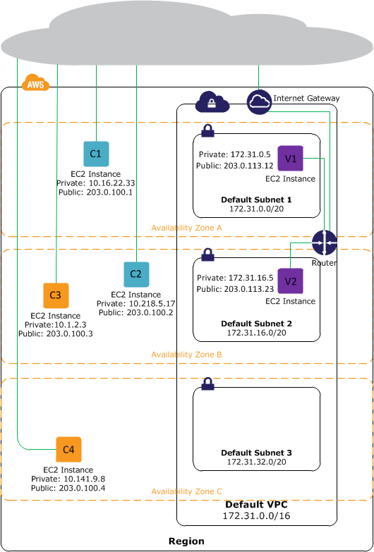
• Instances C1, C2, C3, and C4 are in the EC2-Classic platform. C1 and C2 were launched by one account, and C3 and C4 were launched by a different account. These instances can communicate with each other, can access the Internet directly, and can access other services such as Amazon Simple Storage Service (Amazon S3).

• Instances V1 and V2 are in different subnets in the same VPC in the EC2-VPC platform. They were launched by the account that owns the VPC; no other account can launch instances in this VPC. These instances can communicate with each other and can access the following through the Internet gateway: instances in EC2-Classic, other services (such as Amazon S3), and the Internet.

For more information read the AWS documentation.

Notes regarding SSH

One of the first things that happens when the SSH connection is being established is that the server sends its public key to the client, and proves to the client that it knows the associated private key. The client may check that the server is a known one, and not some rogue server trying to pass off as the right one. SSH provides only a simple mechanism to verify the server's legitimacy: it remembers servers you've already connected to, in the ~/.ssh/known_hosts file on the client machine (there's also a system-wide file /etc/ssh/known_hosts).

The server only lets a remote user log in if that user can prove that they have the right to access that account. One such method, the default way, the user may present the password for the account that he is trying to log into; the server then verifies that the password is correct. In another such method, the user presents a public key and proves that he possesses the private key associated with that public key. This is exactly the same method that is used to authenticate the server, but now the user is trying to prove its identity and the server is verifying it. The login attempt is accepted if the user proves that he knows the private key and the public key is in the account's authorization list (~/.ssh/authorized_keys on the server). See Stackexchange answer for more info.

• The ssh-keygen command results in updating/creating two files, depending on the option that is passed to it. Usually a -t option is passed. If -t rsa option is passed, the two files which are created are: id_rsa and id_rsa.pub; the private and public keys respectively. If you need to change the password or add one, do ssh-keygen -p. See this post for more information about ssh.

• Once the public key is installed on the server, access will be granted with no password question. The user can use scp to copy the public key file from the client to the server.

• ssh -i initiate an ssh connection with the identityfile_ option. This selects a file from which the identity (private key) for public key authentication is read. The default is ~/.ssh/identity for protocol version 1, and ~/.ssh/id_dsa, ~/.ssh/id_ecdsa, ~/.ssh/id_ed25519 and ~/.ssh/id_rsa for protocol version 2.

SSH vs X.509 Certificates

X.509 is a proposed standard used for generating digitally-signed public-key authentication certificates. These certificates can be used for authentication in supporting SSH systems. Not all SSH servers support X.509 certificates.[1]

SSH protocol doesn’t define a standard for storing SSH keys (such as X.509, used in SSL). However, like X.509 certificates, SSH key pairs also have public and private parts and use RSA or DSA algorithms.

How is X.509 used in SSH? X.509 certificates are used as a key storage, i.e. instead of keeping SSH keys in proprietary format, the software keeps X.509 certificates. When SSH key exchange is done, the keys are taken from certificates.[2]

System File Permission

There are several ways by which Unix permissions are represented. The most common form is symbolic notation as shown by ls -l.

• The first character indicates the file type and is not related to permissions.
• The remaining nine characters are in three sets, each representing a class of permissions as three characters.
  • The first set represents the user class.
  • The second set represents the group class.
  • The third set represents the others class.
• Each of the three characters represent the read, write, and execute permissions:
  • r if reading is permitted, - if it is not.
  • w if writing is permitted, - if it is not.
  • x if execution is permitted, - if it is not.

For more information, see the chmod entry in wikipedia to modify the file permission of a file/folders.

Examples

Example 1: Setting up password-less login on OSX

The following steps follow the guidelines given in this post

1. From the client machine, use ssh-keygen to generate a id_rsa and an id_rsa.pub file, if you have not done so already. For more information on generating ssh keys, see this git-hub page.
2. Create a user account (e.g ruser) on the host (server) machine, and set up a password. This password will be used only once - when copying the public key in the next step.
3. Secure copy the public key, id_rsa.pub, from the client machine to the server; using the scp command. For example scp ~/.ssh/id_rsa.pub ruser@10.0.1.15:/Users/ruser. This is when you will be asked for the password of user ruser on the server. The previous command, copies the id_rsa.pub to the home directory of the user, ruser on the server.
4. Create an .ssh directory on the server - if you don't have one already - in the user's home directory on the server; using mkdir ~/.ssh
5. Move the id_rsa.pub to the .ssh/authorized_keys file using mv ~/id_rsa.pub ~/.ssh/authorized_keys
6. Modify the folder/file permission as follows: chmod 700 ~/.ssh and chmod 600 ~/.ssh/authorized_keys.

Notes on chmod:

• chmod 400 file - owner can read file
• chmod 600 file – owner can read and write
• chmod 700 file – owner can read, write and execute

Example 2: logging on to Amazon EC2 instances using SSH.

There are two ways to using ssh to logging in to an EC2 instance. The first, is to upload your own public key to AWS; and the second is to use the .PEM certificates file that amazon creates.

2.1 Using your own public key:

Assuming that you have created a private and a public key pairs, using ssh-keygen, you can use AWS CLI import-key-pair function to upload this keypairs to Amazon. To facilitate this operation to the R-user, we have created a function upload.key part of the AWS.tool R-package to do exactly that.

upload.key("~/.ssh/id_rsa.pub", "awsKey")

This last command, will upload the pubic key defined in id_rsa.pub to the default user's region, and name it awsKey. At this point, the user can launch a new EC2 instance, and associate awsKey with it.

2.2 Using AMAZON certificate key:

The previous example, assumed that the private key was generated using ssh-keygen. As mentioned elsewhere in the document, X.509 certificates like SSH key pairs, also have public and private parts. In this example, we will use the X.509 certificates created from Amazon Web Services (CLI or Console), to log on to an EC2 instances that was initiated with that key pairs.

1. Download the .PEM file from AWS (using either the create-keys command, or AWS console); after having created the certificates.
2. Assuming the name of the downloaded file is my-key-pair.pem; change its permission using chmod 400 my-key-pair.pem

2.2.1 The standard way

As described in AWS documentation to log-in to an instance ssh -i my-key-pair.pem ec2-user@ec2-198-51-100-1.compute-1.amazonaws.com where:

• The public DNS is ec2-198-51-100-1.compute-1.amazonaws.com
• And the user is ec2-user. This username is the default user for Amazon AMI; and should be replaced by ubuntu if you are using an Ubuntu AMI.
• The -i option in the ssh command selects a file from which the identity (private key) for public key authentication is read.

2.2.2 Adding the key to the ssh-agent

For the second approach:

1. Copy the my-key-pair.pem file to the ~/.ssh folder.
2. Add the key to the ssh agent using the following command: ssh-add -K ~/.ssh/my-key-pair.pem.
   • The -K option in the last command, adds your private key to the keychain application in OSX. Whenever you reboot your Mac, all the SSH keys in your keychain will be automatically loaded to the ssh-agent program. Starting from Mac OS X 10.8 and higher, Apple has integrated launchd(8) and Keychain support into ssh-agent(1) so it launches automatically on-demand and can interact with keys stored in Keychain Access.[3]
   • If you do not specify the -K options, you will have to run the ssh-add command everytime you restart the machine. You can put that command in your .profile or .bashrc so they get executed every time you log in

At this point, you can simply type ssh ec2-user@ec2-198-51-100-1.compute-1.amazonaws.com without using the -i option.

Notes on ssh-add from the man page:

• ssh-add -l to see the keys in the ssh-agent,
• ssh-add -D to delete all identity from the agent.
• ssh-add -d to delete a specific identity.

2.2.3 Using a config file for ssh

In this third approach, you create a file called config and you place it in ~/.ssh folder. The content of this file can be as follows:

Host *.compute-1.amazonaws.com
 IdentityFile ~/.ssh/my-key-pair.pem
 User ec2-user

where IdentityFile points to the location to .PEM file, and User would be ubuntu if logging into an Ubuntu instance. For more information on the config file, see this post, and the man page of SSH_CONFIG.

At this point, we can issue the following command ssh ec2-198-51-100-1.compute-1.amazonaws.com, and the identity file and user would be infered from the config file.

Configuration of SSH with Airport extreme

See http://apple.stackexchange.com/questions/39464/remotely-ssh-to-ip-address-in-home-network

In this post, we will use the R-package FRBData, (Takayanagi, 2011) to fetch interest rate data from the internet, plots its term structure, and compute the forward discount count.

Fetching the data

The FRBData package provides functions which can get financial and economical data from Federal Reserve Bank's website. For information regarding the day count convention and the compounding frequency of IR curves, read the footnote on the website.

For example, in order to get the SWAP curve, for a specific range of dates, we would type the following in the the R termial

library(FRBData)

ir_swp_rates <- GetInterestRates(id = "SWAPS",from = as.Date("2014/06/11"), to = as.Date("2014/06/30"))

For the rest of this post, we will use the Constant Maturity Rate

Constant Maturity Rate

CMT yields are read directly from the Treasury's daily yield curve and represent "bond equivalent yields" for securities that pay semiannual interest, which are expressed on a simple annualized basis. As such, these yields are not effective annualized yields or Annualized Percentage Yields (APY), which include the effect of compounding. To convert a CMT yield to an APY you need to apply the standard financial formula:

APY = (1 + CMT/2)^2 -1

Treasury does not publish the weekly, monthly or annual averages of these yields. However, the Board of Governors of the Federal Reserve System also publishes these rates on our behalf in their Statistical Release H.15. The web site for the H.15 includes links that have the weekly, monthly and annual averages for the CMT indexes

Similar to the SWAP rate example above, in order to get the CMT rates into R, we use the following command

# Constant maturity yield curve
ir_const_maturities <- GetInterestRates(id = "TCMNOM",lastObs = 11)

Note that in the above example, instead of specifying a date range, we are opting to fetch the last 11 observations.

Plotting a term structure for a specific day

The following code was inspirerd by the one provided by (Hanson, 2014). For the plot, we will use the R-package ggplot2 (Wickham, 2009)

library(ggplot2)
i <- 10
term_str <- t(ir_const_maturities[i, ])
ad <- index(ir_const_maturities)[i] # anchor date

# Plotting the term structure
df.tmp <- data.frame(term = 1:length(ir_const_maturities[i, ]), rates  = t(coredata(ir_const_maturities[i, ])))
gplot <- ggplot(data = df.tmp, aes(x = term, y = rates)) + geom_line() +geom_point()
gplot <- gplot + scale_x_discrete(breaks=df.tmp$term, labels=colnames(ir_const_maturities))
gplot <- gplot + ggtitle(paste("Market Zero Rates for:", ad)) + xlab("Term") + ylab("Rates (%)")
gplot

Yield Curve Construction

The first step is to construct the term-axis based on the columns names of the obtained data. To facilitate the construction of the various date, we will be using the lubridate package (Grolemund and Wickham, 2011)

library(lubridate)
term.str.dt <- c()
for (j in colnames(ir_const_maturities)) {
  term_num <- as.numeric(substring(j, 1, nchar(j) - 1))
  term <- switch(tolower(substring(j, nchar(j))), 
                 "y" = years(term_num),
                 "m" = months(term_num),
                 "w" = weeks(term_num),
                 stop("Unit unrecognized in the term structure file"))
  term.str.dt <- cbind(term.str.dt, ad + term)
}
term.str.dt <- as.Date(term.str.dt, origin = "1970-01-01")

Next step is we construct the curve for the most recent date

require(xts)
ad <- index(last(ir_const_maturities))
rates <- t(coredata(last(ir_const_maturities))) * 0.01 # converting the decimal from percentage
# Make sure that the data is monotone - it's NOT always the case, since these data are weekly averages and not directly observed
if (any(rates != cummax(rates))) { 
  # Checks if the data is montonoe, if not fix it
  for (t in 2:length(rates)) {
    if (rates[t] < rates[t-1]) rates[t] = rates[t-1]
  } 
}

As mentioned in the above comments, we have to make sure that the IR data is monotonically increasing - otherwise we obtain a negative forward rate which will result in arbitrage opportunity. In order to do so, we cummax function as described in (Ali, 2012)

Next, we will use the xts package (Ryan and Ulrich, 2014) to construct and represent the zero curve

zcurve <- as.xts(x = rates, order.by = term.str.dt)

seq.date <- seq.Date(from = index(last(ir_const_maturities)), to = last(index(zcurve)), by = 1)
term.str.dt.daily <- xts(order.by= seq.date)

zcurve <- merge(zcurve, term.str.dt.daily)

Next we interpolate the data in between. In the following example we will use two interpolation methods: linear and cubic spline

zcurve_linear <- na.approx(zcurve) # Linear interpolation
zcurve_spline <- na.spline(zcurve, method = "hyman") # Spline interpolation which guarentees monotone output
colnames(zcurve_spline) <- NULL
zcurve_spline <- na.locf(zcurve_spline, na.rm = FALSE, fromLast = TRUE) # flat extrapolation to the left

Plotting the interpolated curve

library(scales) # needed for the date_format() function
df.tmp <- data.frame(term = index(zcurve_spline), rates = coredata(zcurve_spline))
gplot <- ggplot(data = df.tmp, aes(x = term, y = rates)) + geom_line()
gplot <- gplot + scale_x_date(labels = date_format())
gplot <- gplot + theme(axis.text.x = element_text(angle = 90, vjust = 0.5, hjust=1))
gplot <- gplot + ggtitle(paste("Market Zero Rates for:", ad)) + xlab("Term") + ylab("Rates (%)")
gplot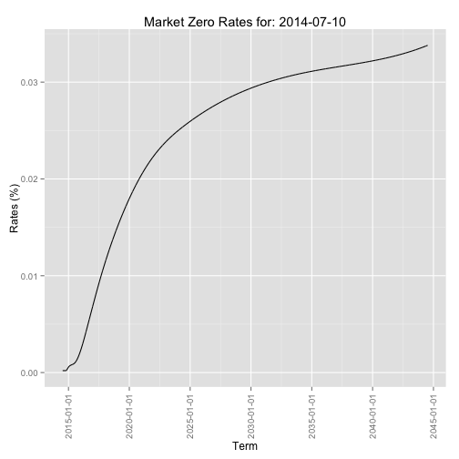

Note: In order to see the impact of using the default cubic spline method, instead of the using method = "hyman", the reader should refer to (Ali, 2012)

Construction of the forward curves and taking Day Count Convention into account

The code for the this section is borrowed from (Hanson, 2014)

First step is the construction of the function that computes the fraction of a year, based on the day count convention of the curve. We illustrate this by construction a code that uses ACT/365 days count convention

delta_t_Act365 <- function(from_date, to_date){
  if (from_date > to_date) 
    stop("the 2nd parameters(to_date) has to be larger/more in the future than 1st paramters(from_date)")
  yearFraction <- as.numeric((to_date - from_date)/365)
  return(yearFraction)  
}

Next we construct the forward discount factor based on the day count convention, and using the function we just defined

fwdDiscountFactor <- function(t0, from_date, to_date, zcurve.xts, dayCountFunction) {
  if (from_date > to_date) 
    stop("the 2nd parameters(to_date) has to be larger/more in the future than 1st paramters(from_date)")
  rate1 <- as.numeric(zcurve.xts[from_date])      # R(0, T1)
  rate2 <- as.numeric(zcurve.xts[to_date])        # R(0, T2)
  # Computing discount factor
  discFactor1 <- exp(-rate1 * dayCountFunction(t0, from_date))
  discFactor2 <- exp(-rate1 * dayCountFunction(t0, to_date))
  
  fwdDF <- discFactor2/discFactor1
  return(fwdDF)
}

Finally we compute the forward zero curve, again using the day count convention function we have defined above

fwdInterestRate <- function(t0, from_date, to_date, zcurve.xts, dayCountFunction) {
  # we are passing the zero curve, because we will compute the discount factor inside this function
  if (from_date > to_date) 
    stop("the 2nd parameters(to_date) has to be larger/more in the future than 1st paramters(from_date)")
  else if (from_date == to_date)
    return(0)
  else {
    fwdDF <- fwdDiscountFactor(t0, from_date, to_date, zcurve.xts, dayCountFunction)
    fwdRate <- -log(fwdDF)/dayCountFunction(from_date, to_date)
  }
  return(fwdRate)
}

Examples

Putting it all together, in order to use the above code to compute the forward discount factor/rate, observed at time t0, we would use the following code

t0 <- index(last(ir_const_maturities))

fwDisc <- fwdDiscountFactor(t0, from_date = t0 + years(5), to_date = t0 + years(10), 
                            zcurve.xts = zcurve_spline, dayCountFunction = delta_t_Act365)

fwrate <- fwdInterestRate(t0, from_date = t0 + years(5), to_date = t0 + years(10), 
                          zcurve.xts = zcurve_spline, dayCountFunction = delta_t_Act365)

Validation examples:

# Test 1: Trivial case

fwdDiscountFactor(t0, from_date = t0 + years(5), to_date = t0 + years(5), 
                  zcurve.xts = zcurve_spline, dayCountFunction = delta_t_Act365)

## [1] 1

fwdInterestRate(t0, from_date = t0 + years(5), to_date = t0 + years(5), 
                zcurve.xts = zcurve_spline, dayCountFunction = delta_t_Act365)

## [1] 0

# Test 2: Recovering the original interest rate

setting the start date to equal t0

tt1 <- fwdInterestRate(t0, from_date = t0, to_date = t0 + months(1), 
                       zcurve.xts = zcurve_spline, dayCountFunction = delta_t_Act365)
tt2 <- coredata(last(ir_const_maturities))[,"1M"] * 0.01 # since the orginial was in decimal format

Checking that the two values are "equal"

all.equal(tt1, tt2, check.attributes = FALSE, tolerance = .Machine$double.eps)

## [1] "Mean relative difference: 1.458e-12"

This value is accurate enough and is smaller than the default threshold of all.equal function

References

Citations made with knitcitations (Boettiger, 2014).

[1] Ali. How to check if a sequence of numbers is monotonically increasing (or decreasing)?. 2012. URL: http://stackoverflow.com/questions/13093912/how-to-check-if-a-sequence-of-numbers-is-monotonically-increasing-or-decreasing.

[2] C. Boettiger. knitcitations: Citations for knitr markdown files. R package version 1.0-1. 2014. URL: https://github.com/cboettig/knitcitations.

[3] G. Grolemund and H. Wickham. "Dates and Times Made Easy with lubridate". In: Journal of Statistical Software 40.3 (2011), pp. 1-25. URL: http://www.jstatsoft.org/v40/i03/.

[4] D. Hanson. Quantitative Finance Applications in R - 6: Constructing a Term Structure of Interest Rates Using R (Part 1). 2014. URL: http://blog.revolutionanalytics.com/2014/06/quantitative-finance-applications-in-r-6-constructing-a-term-structure-of-interest-rates-using-r-par.html.

[5] D. Hanson. Quantitative Finance applications in R - 7: Constructing a Term Structure of Interest Rates Using R (part 2 of 2). 2014. URL: http://blog.revolutionanalytics.com/2014/07/quantitative-finance-applications-in-r-7-constructing-a-term-structure-of-interest-rates-using-r-par.html.

[6] J. A. Ryan and J. M. Ulrich. xts: eXtensible Time Series. R package version 0.9-7. 2014. URL: http://CRAN.R-project.org/package=xts.

[7] S. Takayanagi. FRBData: Download interest rate data from FRB's website. R package version 0.3. 2011. URL: http://CRAN.R-project.org/package=FRBData.

[8] H. Wickham. ggplot2: elegant graphics for data analysis. Springer New York, 2009. ISBN: 978-0-387-98140-6. URL: http://had.co.nz/ggplot2/book.

Reproducibility

sessionInfo()

## R version 3.1.1 (2014-07-10)
## Platform: x86_64-apple-darwin10.8.0 (64-bit)
## 
## locale:
## [1] en_CA.UTF-8/en_CA.UTF-8/en_CA.UTF-8/C/en_CA.UTF-8/en_CA.UTF-8
## 
## attached base packages:
## [1] stats     graphics  grDevices utils     datasets  methods   base     
## 
## other attached packages:
##  [1] scales_0.2.4        lubridate_1.3.3     ggplot2_1.0.0      
##  [4] FRBData_0.3         xts_0.9-7           zoo_1.7-11         
##  [7] bibtex_0.3-6        knitr_1.6           RefManageR_0.8.2   
## [10] knitcitations_1.0-1
## 
## loaded via a namespace (and not attached):
##  [1] codetools_0.2-8  colorspace_1.2-4 digest_0.6.4     evaluate_0.5.5  
##  [5] formatR_0.10     grid_3.1.1       gtable_0.1.2     httr_0.3        
##  [9] labeling_0.2     lattice_0.20-29  MASS_7.3-33      memoise_0.2.1   
## [13] munsell_0.4.2    plyr_1.8.1       proto_0.3-10     Rcpp_0.11.2     
## [17] RCurl_1.95-4.1   reshape2_1.4     RJSONIO_1.2-0.2  stringr_0.6.2   
## [21] tools_3.1.1      XML_3.98-1.1